Guvenen (2009): Asset Pricing with Heterogeneous IES
Guvenen (2009) constructs a two-agent model to account for several salient features of asset pricing moments, such as high risk premium, low and relatively smooth interest rate, and countercyclical movements in risk premium and Sharpe ratio. The two key ingredients of his model are limited stock market participation and heterogeneity in the elasticity of inter-temporal substitution in consumption (EIS).
When all endogenous states are pre-determined, such as capital and bond share in the current example, the expectation of future variables can be parameterized and integrated before solving the system of equilibrium equations, which greatly speeds up the computation. We illustrate how to use parameterized expectation with the toolbox in this example.
The Model
There are two types of infinitely-lived agents: stockholders (\(h\)) with measure \(\mu\), and non-stockholders (\(n\)) with measure \(1-\mu\). Agents have Epstein-Zin utility functions
for \(i=h,n\). Most importantly, \(\rho^{h}<\rho^{n}\), i.e., the non-stockholders have lower EIS which is inversely proportional to \(\rho^{i}\), and thus they have higher desire for consumption smoothness over time. Each agent has one unit of labor endowment.
Stockholders can trade stock \(s_{t}\) and bond \(b_{h,t}\) at prices \(P_{t}^{s}\) and \(P_{t}^{f}\) respectively. Their budget constraint is
where \(W_t\) is the labor income and borrowing constraint is
and in calibration \(\underline{B}\) is set to six times of the average monthly wage rate. The non-stockholders have the same constraints. In addition, they are restricted from trading stocks.
A representative firm produces the consumption good using capital \(K_{t}\) and labor \(L_{t}\) based on a Cobb-Douglas production function:
and the technology evolves according to an AR(1) process:
The firm maximizes its value \(P_{t}^{s}\) expressed as the sum of its future dividends \(\left\{ D_{t+j}\right\} _{j=1}^{\infty}\) discounted by the shareholders’ marginal rate of substitution process:
The firm accumulates capital subject to a concave adjustment cost function in investment:
Each period, the firm sells one-period bonds at price \(P_{t}^{f}\). The bond supply is constant and equals to \(\chi\) fraction of its average capital stock \(\bar{K}\). Thus dividend \(D_{t}\) can be written as
A sequential competitive equilibrium is given by sequences of allocations \(\{c_{i,t},b_{i,t+1},s_{t+1},I_{t},K_{t+1},L_{t}\}\) \(i=h,n\) and prices \(\left\{ P_{t}^{s},P_{t}^{f},W_{t}\right\}\) such that (i) given the price sequences, \(\left\{ c_{i,t},b_{i,t+1},s_{t+1}\right\}\) \(i=h,n\) solve the stockholders’ and non-stockholders’ optimization problems; (ii) Given the wage sequence \(\left\{ W_{t}\right\}\) and the law of motion for capital, \(\left\{L_{t},I_{t}\right\}\) are optimal for the representative firm; (iii) all markets clear:
We compute a recursive equilibrium using \(\left\{ K_{t},B_{t}^{n},Z_{t}\right\}\) as the aggregate state variables, where \(B_{t}^{n}=\left(1-\mu\right)b_{n,t}\) is total bond holding by the non-stockholders. We have \(8\) unknowns: {\(c_{h,t}\), \(c_{n,t}\), \(I_{t}\), \(B_{t+1}^{n}\), \(\lambda_{h,t}\), \(\lambda_{n,t}\), \(P_{t}^{s}\), \(P_{t}^{f}\)}, and the \(8\) equations used to solve them are:
Euler equations for bond holding:
Euler equations for the stockholders’ demand of equity:
Slackness condition of borrowing limit:
The budget constraints (imposing \(s_{t+1}=1/\mu\)):
Firm’s optimal capital accumulation \(K_{t+1}\):
in which capital price \(q_{t}\) is the Lagrangian multiplier on the capital formation equation and satisfies
The auxiliary variables can be determined by the utility function, market clearing conditions, and the following two equations:
In period \(t\), the 6 future variables in use: \(c_{h,t+1}\), \(c_{n,t+1}\), \(P_{t+1}^{s}+D_{t+1}\), \(I_{t+1}/K_{t+1}\), \(U_{h,t+1}\) and \(U_{n,t+1}\) are functions of \(\left\{ K_{t+1},B_{t+1}^{n},Z_{t+1}\right\}\) and are solved from the previous iteration. Similar to Guvenen (2009), the initial guesses for these functions are obtained by solving a version of the model with no leverage.
The gmod File
The model can be solved with the following guvenen2009.gmod file
  1% Parameters
  2parameters beta alpha rhoh rhon theta delta mu xsi chi a1 a2 Kss Bbar bn_shr_lb bn_shr_ub varianceScale;
  3
  4beta = 0.9966;      % discount factor
  5alpha = 6;          % risk aversion
  6rhoh = 1/.3;        % inv IES for stockholders
  7rhon = 1/.1;        % inv IES for non-stockholders
  8theta = .3;         % capital share
  9delta = .0066;      % depreciation rate
 10mu = .2;            % participation rate
 11xsi = .4;           % adjustment cost coefficient
 12chi = .005;         % leverage ratio
 13a1 = (((delta^(1/xsi))*xsi)/(xsi-1));
 14a2 = (delta/(1-xsi));
 15Kss = ((1/beta-1+delta)/theta)^(1/(theta-1));
 16Bbar = -0.1*(1-theta)*Kss^theta; %borrowing constraint
 17varianceScale = 1e4;
 18
 19TolEq = 1e-4;
 20INTERP_ORDER = 4; EXTRAP_ORDER = 4;
 21PrintFreq = 100;
 22SaveFreq = inf;
 23
 24% Shocks
 25var_shock Z;
 26shock_num = 15;
 27phi_z = 0.984;  % productivity AR(1)
 28mu_z = 0;
 29sigma_e = 0.015/(1+phi_z^2+phi_z^4).^0.5;
 30[z,shock_trans,~]=tauchen(shock_num,mu_z,phi_z,sigma_e,2);
 31Z = exp(z);
 32
 33% States
 34var_state K bn_shr;
 35K_pts = 10;
 36K = exp(linspace(log(.84*Kss),log(1.2*Kss),K_pts));
 37
 38bn_shr_lb = (1-mu)*Bbar/(chi*Kss);
 39bn_shr_ub = (chi*Kss - mu*Bbar)/(chi*Kss);
 40b_pts = 30;
 41bn_shr = linspace(bn_shr_lb,bn_shr_ub,b_pts);
 42
 43% Last period
 44var_policy_init c_h c_n;
 45
 46inbound_init c_h 1e-6 100;
 47inbound_init c_n 1e-6 100;
 48
 49var_aux_init Y W vh vn vhpow vnpow Ps Pf Div Eulerstock Eulerbondh Eulerbondn Inv dIdK Eulerf;
 50
 51model_init;
 52  Y = Z*(K^theta);
 53  W = (1-theta)*Z*(K^theta);
 54  resid1 = 1 - (W + (bn_shr*chi*Kss/(1-mu)))/c_n; % c_n: individual consumption
 55  resid2 = 1 - (W + (Div/mu) + ((1-bn_shr)*chi*Kss/mu))/c_h; % c_h: individual consumption
 56  vh = ((1-beta)*(c_h^(1-rhoh)))^(1/(1-rhoh));
 57  vn = ((1-beta)*(c_n^(1-rhon)))^(1/(1-rhon));
 58  vhpow = vh^(1-alpha);
 59  vnpow = vn^(1-alpha);
 60  Pf = 0;
 61  Ps = 0;
 62  Div = Y - W - (1-Pf)*chi*Kss;  % investment is zero
 63
 64  Eulerstock = (vh^(rhoh-alpha))*(c_h^-rhoh)*(Ps + Div);
 65  Eulerbondh = (vh^(rhoh-alpha))*(c_h^-rhoh);
 66  Eulerbondn = (vn^(rhon-alpha))*(c_n^-rhon);
 67
 68  Inv = 0;
 69  Knext = 0;
 70  dIdK = (Inv/K) - (1/a1)*(xsi/(xsi-1))*(Inv/(K*((1/a1)*((Knext/K)-(1-delta)-a2))))*(Knext/K);
 71  Eulerf = (vh^(rhoh-alpha))*(c_h^-rhoh)*(theta*Z*(K^(theta-1)) - dIdK);
 72
 73  equations;
 74     resid1;
 75     resid2;
 76  end;
 77end;
 78
 79var_interp EEulerstock_interp EEulerbondh_interp EEulerbondn_interp EEulerf_interp Evh_interp Evn_interp EPD_interp EPD_square_interp;
 80initial EEulerstock_interp shock_trans*reshape(Eulerstock,shock_num,[]);
 81initial EEulerbondh_interp shock_trans*reshape(Eulerbondh,shock_num,[]);
 82initial EEulerbondn_interp shock_trans*reshape(Eulerbondn,shock_num,[]);
 83initial EEulerf_interp shock_trans*reshape(Eulerf,shock_num,[]);
 84initial Evh_interp shock_trans*reshape(vhpow,shock_num,[]);
 85initial Evn_interp shock_trans*reshape(vnpow,shock_num,[]);
 86initial EPD_interp shock_trans*reshape(Div,shock_num,[]);
 87initial EPD_square_interp shock_trans*reshape(Div.^2,shock_num,[]) / varianceScale;
 88
 89EEulerstock_interp = shock_trans*Eulerstock;
 90EEulerbondh_interp = shock_trans*Eulerbondh;
 91EEulerbondn_interp = shock_trans*Eulerbondn;
 92EEulerf_interp = shock_trans*Eulerf;
 93Evh_interp = shock_trans*vhpow;
 94Evn_interp = shock_trans*vnpow;
 95EPD_interp = shock_trans*(Ps+Div);
 96EPD_square_interp = shock_trans*(Ps+Div).^2 / varianceScale;
 97
 98% Endogenous variables, bounds, and initial values
 99var_policy c_h c_n Ps Pf Inv bn_shr_next lambdah lambdan;
100
101inbound c_h 1e-3 10;
102inbound c_n 1e-3 10;
103inbound Ps 1e-3 500;
104inbound Pf 1e-3 10;
105inbound Inv 1e-9 10;
106inbound bn_shr_next bn_shr_lb bn_shr_ub;
107inbound lambdah 0 2;
108inbound lambdan 0 2;
109
110% Other equilibrium variables
111var_aux Y W b_h b_n Div dIdKp Eulerstock Eulerbondh Eulerbondn dIdK Eulerf vhpow vnpow omega PDratio Rs R_ep vh vn Knext std_ExcessR SharpeRatio;
112
113model;
114  Y = Z*(K^theta);              % output
115  W = (1-theta)*Z*(K^theta);    % Wage = F_l
116  Div = Y - W - Inv - (1-Pf)*chi*Kss;            % dividends
117
118  Knext = (1-delta)*K + (a1*((Inv/K)^((xsi-1)/xsi))+a2)*K;
119  dIdKp = (1/a1)*(xsi/(xsi-1))*(Inv/(K*((1/a1)*((Knext/K)-(1-delta)-a2))));
120
121  b_h = (1-bn_shr)*chi*Kss/mu;
122  b_n = bn_shr*chi*Kss/(1-mu);
123
124  [EEulerstock_future,EEulerbondh_future,EEulerbondn_future,EEulerf_future,Evh_future,Evn_future,EPD_future,EPD_square_future] = GDSGE_INTERP_VEC(shock,Knext,bn_shr_next);
125  EPD_square_future = EPD_square_future*varianceScale;
126
127  vh =  ((1-beta)*(c_h^(1-rhoh)) + beta*(Evh_future^((1-rhoh)/(1-alpha))))^(1/(1-rhoh));
128  vn =  ((1-beta)*(c_n^(1-rhon)) + beta*(Evn_future^((1-rhon)/(1-alpha))))^(1/(1-rhon));
129
130  Eulerstock = (vh^(rhoh-alpha))*(c_h^-rhoh)*(Ps + Div);
131  Eulerbondh = (vh^(rhoh-alpha))*(c_h^-rhoh);
132  Eulerbondn = (vn^(rhon-alpha))*(c_n^-rhon);
133
134  dIdK = (Inv/K) - (1/a1)*(xsi/(xsi-1))*(Inv/(K*((1/a1)*((Knext/K)-(1-delta)-a2))))*(Knext/K);
135  Eulerf = (vh^(rhoh-alpha))*(c_h^-rhoh)*(theta*Z*(K^(theta-1)) - dIdK);
136
137  vhpow = vh^(1-alpha);
138  vnpow = vn^(1-alpha);
139
140  omega = (Ps+Div+ mu*b_h)/(Ps+Div+chi*Kss);
141  PDratio = Ps/Div;
142  Rs = EPD_future/Ps;
143  R_ep = Rs - 1/Pf;
144  % The following inline implements
145  % std_ExcessR = (GDSGE_EXPECT{(PD_future'/Ps - Rs)^2})^0.5;
146  std_ExcessR = (EPD_square_future/(Ps^2) + Rs^2 - 2*EPD_future*Rs/Ps)^0.5;
147  SharpeRatio = R_ep/std_ExcessR;
148
149  % Equations:
150  err_bdgt_h = 1 - (W + (Div/mu) + b_h - Pf*(chi*Kss*(1-bn_shr_next)/mu))/c_h; % these are individual consumptions
151  err_bdgt_n = 1 - (W + b_n - Pf*(bn_shr_next*chi*Kss/(1-mu)))/c_n;
152  foc_stock = 1 - (beta*EEulerstock_future*(Evh_future^((alpha-rhoh)/(1-alpha))))/((c_h^(-rhoh))*Ps);
153  foc_bondh = 1 - (beta*EEulerbondh_future*(Evh_future^((alpha-rhoh)/(1-alpha))) + lambdah)/((c_h^(-rhoh))*Pf);
154  foc_bondn = 1 - (beta*EEulerbondn_future*(Evn_future^((alpha-rhon)/(1-alpha))) + lambdan)/((c_n^-rhon)*Pf);
155  foc_f = 1 - (beta*EEulerf_future*(Evh_future^((alpha-rhoh)/(1-alpha))))/((c_h^(-rhoh))*dIdKp);
156
157  slack_bn = lambdan*(bn_shr_next - bn_shr_lb);    %mun_lw*bn_shr_next;
158  slack_bh = lambdah*(bn_shr_ub - bn_shr_next);    %mun_up*(1-bn_shr_next);
159
160  equations;
161    err_bdgt_h;
162    err_bdgt_n;
163    foc_stock;
164    foc_bondh;
165    foc_bondn;
166    foc_f;
167    slack_bn;
168    slack_bh;
169  end;
170
171end;
172
173simulate;
174  num_periods = 10000;
175  num_samples = 100;
176
177  initial K Kss;
178  initial bn_shr 0.5;
179  initial shock 2;
180
181  var_simu Y c_h c_n Inv Ps Div Pf bn_shr_next Knext omega PDratio Rs R_ep SharpeRatio std_ExcessR;
182
183  K' = Knext;
184  bn_shr' = bn_shr_next;
185end;
The implementation uses the exact parameterization and specification (number of grid points, domains of endogenous state variables, number of discretized exogenous shocks, the cubic spline approximation, etc.) in Guvenen (2009). However, the algorithm differs from his. His is based on the algorithm in Krusell and Smith (1998): starting from a conjectured law of motion for state-variables and pricing functions, he solves the agents’ Bellman equation and the agents’ policy functions using standard value function iterations. Then he uses these policy functions and temporary market clearing conditions to obtain a new law of motions and new pricing functions. The current algorithm, like other examples, utilizes the fact that agents’ optimization is concave, replaces the agent’s optimization with first order and complementarity conditions, and solves the agents’ optimization problem together with the market clearing conditions.
Since both state variables \(K_t\) and \(B_t^n\) are predetermined, the expectation of future variables (e.g., the marginal utility entering the bond’s Euler equation, or the price and dividend entering the equity’s Euler equation) can be calculated before-hand conditional on current exogenous states. For example, for the bond’s Euler equation
we can define function
and approximate \(\tilde{\Lambda}(z,K',B')\) instead of \(\Lambda(z',K',B')\). This is made possible by that \((K,B)\) are predetermined in that the transition of the two states do not depend on \(z'\) (this is not true when the endogenous state follows an implicit state transition function that depends on the realization of \(z'\), such as wealth share and consumption share). When a projection method or spline is used to approximate \(\tilde{\Lambda}(z,K,B)\), the integration becomes quite simple, since projection is a linear operator and therefore the projection of an expectation equals to the expectation of the projection.
Once \(\tilde{\Lambda}(z,K',B')\) is approximated beforehand, then one only needs to evaluate \(\tilde{\Lambda}\) once for the current exogenous shock (\(z\)) in each evaluation of the system of equations. If instead one is to work with \(\Lambda(z',K',B')\), \(\Lambda\) needs to be evaluated for each \(z'\) and integrated using the transition matrix. This is why integrating \(\Lambda(z',K',B')\) beforehand is more computation-efficient, especially when the size of exogenous shocks is large.
In particular, the parameterized expectation is implemented by declaring the expectation of relevant variables in var_interp in
79var_interp EEulerstock_interp EEulerbondh_interp EEulerbondn_interp EEulerf_interp Evh_interp Evn_interp EPD_interp EPD_square_interp;
specifying the updating of var_interp by integrating the corresponding variables using the transition matrix
89EEulerstock_interp = shock_trans*Eulerstock;
90EEulerbondh_interp = shock_trans*Eulerbondh;
91EEulerbondn_interp = shock_trans*Eulerbondn;
92EEulerf_interp = shock_trans*Eulerf;
93Evh_interp = shock_trans*vhpow;
94Evn_interp = shock_trans*vnpow;
95EPD_interp = shock_trans*(Ps+Div);
96EPD_square_interp = shock_trans*(Ps+Div).^2 / varianceScale;
and evaluating the approximation at the current shock only when evaluating the system of equations
124 [EEulerstock_future,EEulerbondh_future,EEulerbondn_future,EEulerf_future,Evh_future,Evn_future,EPD_future,EPD_square_future] = GDSGE_INTERP_VEC(shock,Knext,bn_shr_next);
where the GDSGE_INTERP_VEC takes the first argument shock, a reserved keyword referring to the index of the current exogenous shock.
After processed by the online compiler, we can run the returned file to run policy iterations:
>> options = struct;
options.MaxIter = 500;
IterRslt = iter_guvenen2009(options);

Iter:100, Metric:0.512539, maxF:8.65033e-09
Elapsed time is 8.272149 seconds.
Iter:200, Metric:0.285722, maxF:9.39891e-09
Elapsed time is 7.549686 seconds.
Iter:300, Metric:0.174423, maxF:9.01752e-09
Elapsed time is 7.250628 seconds.
Iter:400, Metric:0.113139, maxF:8.89712e-09
Elapsed time is 6.938417 seconds.
Iter:500, Metric:0.0763611, maxF:8.61954e-09
Elapsed time is 6.762700 seconds.
We first solve a simple version of the problem as a warm-up. This simple problem has a lower aggregate net supply of bond (\(\chi=0.005\)) and a tighter borrowing constraint (\(\bar{B}\)). This ensures that starting from a last period solution the equilibrium exists, which is also noted in Guvenen (2009).
Starting with the warm-up solution, we now change the parameters, increase \(\chi\) to \(0.15\), its value in the paper, and specify a much more relaxed borrowing constraint (\(\bar{B}\)). This can be done very conveniently with the toolbox by specifying the new parameters into a structure, and the warm-up solution as a field named WarmUp into the structure.
>> beta = 0.9967;      % discount factor
theta = .3;         % capital share
delta = .0066;      % depreciation rate
mu = .2;            % participation rate
Kss = ((1/beta-1+delta)/theta)^(1/(theta-1));
chi = 0.15;
Bbar = -6*(1-theta)*Kss^theta;
bn_shr_lb = (1-mu)*Bbar/(chi*Kss);
bn_shr_ub = (chi*Kss - mu*Bbar)/(chi*Kss);
b_pts = 30;

options = struct;
options.chi = chi;
options.Bbar = Bbar; %borrowing constraint
options.bn_shr_lb = bn_shr_lb;
options.bn_shr_ub = bn_shr_ub;
options.bn_shr = linspace(bn_shr_lb,bn_shr_ub,b_pts);

options.WarmUp = IterRslt;
options.SkipModelInit=1;
We can now call the routine with the option structure as an argument
>> IterRslt = iter_guvenen2009(options);

Iter:600, Metric:0.0605821, maxF:9.85466e-09
Elapsed time is 6.361178 seconds.

...

Iter:2490, Metric:9.99635e-05, maxF:9.29708e-09
Elapsed time is 5.205234 seconds.
The policy iteration continues from where the warm-up solution ends, toward convergence.
We can inspect the policy functions at convergence by calling in MATLAB:
figure; clf;
subplot(1,2,1);
surf(KMesh,BMesh,squeeze(var_aux.R_ep(z1,:,:))*12);
title('Equity Premium');
xlabel('$K$','Interpreter','Latex');
ylabel('$B_n$','Interpreter','Latex');
set(gca,'FontSize',15);

subplot(1,2,2);
surf(KMesh,BMesh,squeeze((1./var_policy.Pf(z1,:,:))-1)*12);
title('Interest Rate');
xlabel('$K$','Interpreter','Latex');
ylabel('$B_n$','Interpreter','Latex');
set(gca,'FontSize',15);
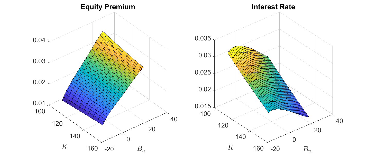
As shown, given capital, as the bond holding of non-stock holders increases, the demand for bond increases and for stock decreases, which results in a lower interest rate, lower stock price and lower equity premium.
We can then simulate the economy
>> SimuRslt = simulate_guvenen2009(IterRslt);
Periods: 1000
shock       K  bn_shr       Y     c_h     c_n     Inv      Ps     Div      Pfbn_shr_next   Knext   omega PDratio      Rs    R_epSharpeRatio
    8   126.1  0.3264   4.267   5.103   3.003  0.8448   111.7  0.3939  0.9978  0.3265   126.1  0.9521   283.7   1.0040.002244 0.04976
Elapsed time is 28.379607 seconds.
Periods: 2000
shock       K  bn_shr       Y     c_h     c_n     Inv      Ps     Div      Pfbn_shr_next   Knext   omega PDratio      Rs    R_epSharpeRatio
    9   127.3  0.3652   4.341   5.197    3.04   0.869   119.3  0.4121  0.9989  0.3655   127.3  0.9493   289.5   1.003 0.00224 0.05007
Elapsed time is 25.144899 seconds.
Periods: 3000
shock       K  bn_shr       Y     c_h     c_n     Inv      Ps     Div      Pfbn_shr_next   Knext   omega PDratio      Rs    R_epSharpeRatio
    11   135.2  0.5826   4.547   5.381   3.158  0.9444   136.5  0.4421   1.001  0.5829   135.3   0.928   308.7   1.0010.002332 0.05232
Elapsed time is 14.973382 seconds.
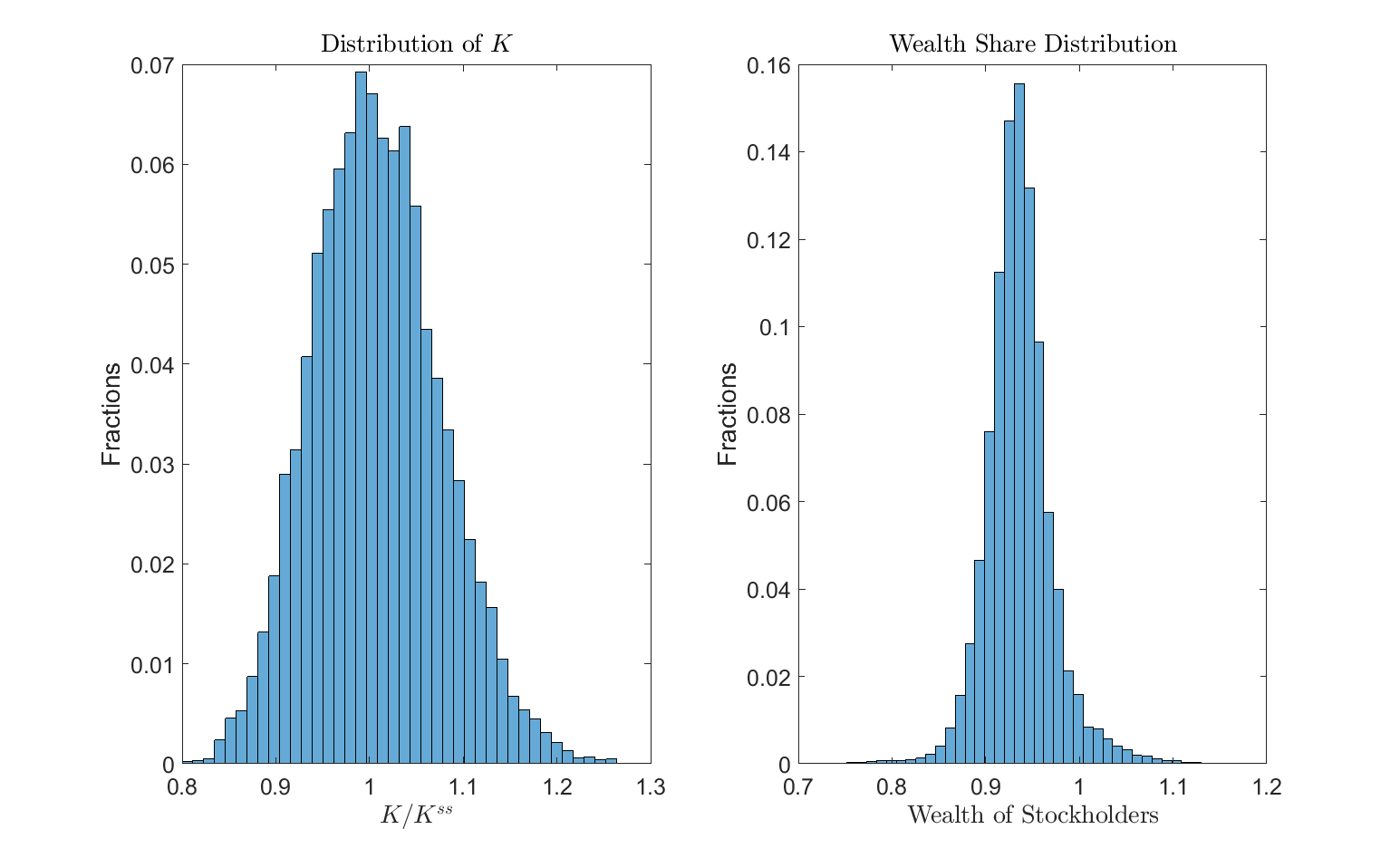
and inspect the distribution of state variables in the ergodic set
startPeriods = 500;
Kss = IterRslt.params.Kss;
K = SimuRslt.K(:,startPeriods:end);
omega = SimuRslt.omega(:,startPeriods:end);

figure; clf;
subplot(1,2,1);
histogram(K/Kss,40,'Normalization','probability');%,'BinLimits',[0.5,0.75]);
title('Distribution of $K$','Interpreter','Latex');
xlabel('$K/K^{ss}$','Interpreter','Latex');
ylabel('Fractions');
set(gca,'FontSize',15);

subplot(1,2,2);
histogram(omega,40,'Normalization','probability');%,'BinLimits',[0.5,0.75]);
title('Wealth Share Distribution','Interpreter','Latex');
xlabel('Wealth of Stockholders','Interpreter','Latex');
ylabel('Fractions');
set(gca,'FontSize',15);
What’s Next?
This example illustrates how to work with parameterized expectation with the toolbox, which greatly reduces computation cost for models that can be solved with predetermined endogenous state variables. The finite-agent asset pricing model is an important class in the Macro and Macro-finance literature. Since the framework of the toolbox solves allocations and prices jointly respecting the optimality and market clearing conditions, it is able to deal with setups which are traditionally regarded as ill-conditioned, such as models with very high risk aversion levels (see example Barro et al. (2017)) or models with equilibrium asset returns that are close to collinear such as Cao, Evans, and Luo (2020).
Or you can directly proceed to Toolbox API.