Getting Started - A Simple RBC Model

The Model

The model is a canonical complete-markets Real Business Cycle (RBC) model with a single productivity shock. This simple model can be approximated with linear solutions well, so using GDSGE to obatin global non-linear solutions is not necessary. Nevertheless it serves as a good starting point to illustrate the basic usage of the toolbox, as this model should be familiar to any macroeconomic audience.

Time is discrete \(t=0...\infty\). Representative households with mass one maximize utility

\[\mathbb E \sum_{t=0}^{\infty} \beta^t \frac{c_t^{1-\sigma}}{1-\sigma},\]

where parameter \(\beta>0\) is the discount factor, \(\sigma>0\) is the coefficient of relative risk aversion. \(c_t\) is the consumption. \(\mathbb{E}\) is an expectation operator integrating the productivity shock to be introduced below.

Competitive representative firms produce a single output according to

\[Y_t=z_t K_t^{\alpha} L_t^{1-\alpha},\]

where parameter \(\alpha \in (0,1)\) is the capital share. \(K_t\) is capital, \(L_t\) is labor, and \(z_t\in\{z_L,z_H\}\) is the productivity shock which follows a two-point Markov process with the following transition matrix

\[\begin{split}\left( \begin{aligned} \pi_{LL} \quad 1-\pi_{LL}\\ 1-\pi_{HH} \quad \pi_{HH} \end{aligned} \right).\end{split}\]

Capital depreciates at rate \(\delta \in (0,1)\). Investment technology can convert one unit of output to new capital:

\[K_{t+1} = K_t(1-\delta) + I_t.\]

Assets markets are complete. Households make investment decision and supply capital and labor to firms. Market clearing conditions for labor and goods are, respectively,

\[\begin{split}L_t=1, \\ c_t+I_t=Y_t.\end{split}\]

The complete-markets equilibrium can be characterized by the Euler equation and the goods market clearing condition:

(1)\[\begin{split}c_t^{-\sigma}=\beta \mathbb{E}_t \left[\left ( \alpha z_{t+1} K_{t+1}^{\alpha-1}+(1-\delta)\right)c_{t+1}^{-\sigma}\right], \\ c_t+K_{t+1} = z_tK_t^{\alpha}+(1-\delta)K_t.\end{split}\]

Given \(K_0\), a sequential competitive equilibrium is stochastic processes \((c_t,K_{t+1})\) that satisfy system (1). To input the system into GDSGE, we need to write the system in a recursive form.

Definition: a recursive competitive equilibrium is functions \(c(z,K), K'(z,K)\) s.t.

\[\begin{split}c(z,K)^{-\sigma}=\beta \mathbb{E}\left[ \left (\alpha z' [K'(z,K)]^{\alpha-1}+(1-\delta)\right)[c(z',K'(z,K))]^{-\sigma} \Big| z \right] \\ c(z,K)+K'(z,K)=zK^{\alpha} + (1-\delta)K.\end{split}\]

The recursive system can be solved using a time iteration procedure:

\[\begin{split}c_t(z,K)^{-\sigma}=\beta \mathbb{E}\left[ \left (\alpha z' [K_t'(z,K)]^{\alpha-1}+(1-\delta)\right)[c_{t+1}(z',K_t'(z,K))]^{-\sigma} \Big| z \right] \\ c_t(z,K)+K'_t(z,K)=zK^{\alpha} + (1-\delta)K.\end{split}\]

taking function \(c_{t+1}(z,K)\) as known in the period-\(t\) time step.

The gmod File

The recursive system can now be input to GDSGE via a mod file rbc.gmod below.

% Parameters
parameters beta sigma alpha delta;
beta  = 0.99;		% discount factor
sigma = 2.0;		% CRRA coefficient
alpha = 0.36;		% capital share
delta = 0.025;		% depreciation rate

% Exogenous States
var_shock z;
shock_num = 2;
z_low = 0.99; z_high = 1.01;
Pr_ll = 0.9;  Pr_hh  = 0.9;
z = [z_low,z_high];
shock_trans = [
  Pr_ll, 1-Pr_ll
  1-Pr_hh, Pr_hh
  ];

% Endogenous States
var_state K;
Kss  = (alpha/(1/beta - 1 + delta))^(1/(1-alpha));
KPts = 101;
KMin = Kss*0.9;
KMax = Kss*1.1;
K    = linspace(KMin,KMax,KPts);

% Interp
var_interp c_interp;
initial c_interp z.*K.^alpha+(1-delta)*K;
% Time iterations update
c_interp = c;

% Endogenous variables as unknowns of equations
var_policy c K_next;
inbound c       0 z.*K.^alpha+(1-delta)*K;
inbound K_next  0 z.*K.^alpha+(1-delta)*K;

% Other endogenous variables
var_aux w;

model;
  % Budget constraints
  u_prime = c^(-sigma);
  kret_next' = z'*alpha*K_next^(alpha-1) + 1-delta;
  
  % Evaluate the interpolation object to get future consumption
  c_future' = c_interp'(K_next);
  u_prime_future' = c_future'^(-sigma);
  
  % Calculate residual of the equation
  euler_residual = 1 - beta*GDSGE_EXPECT{u_prime_future'*kret_next'}/u_prime;
  market_clear = z*K^alpha + (1-delta)*K - c - K_next;
  
  % Calcualte other endogenous variables
  w = z*(1-alpha)*K^alpha;
  
  equations;
    euler_residual;
    market_clear;
  end;
end;

simulate;
  num_periods = 10000;
  num_samples = 6;
  initial K Kss;
  initial shock 1;
  var_simu c K w;
  K' = K_next;
end;

The gmod file can be uploaded to the online compiler at http://www.gdsge.com/ (Remember also to download the necessary runtime files following the instruction on the compiler website). The compiler returns three files that can be used to solve and simulate the model: iter_rbc.m, simulate_rbc.m, mex_rbc.mexw64.

First, call iter_rbc.m in matlab to run the policy iterations and store the returned result in IterRslt, which produces

>> IterRslt = iter_rbc;

Iter:10, Metric:0.385607, maxF:9.99011e-09
Elapsed time is 0.174117 seconds.

...

Iter:323, Metric:9.89183e-07, maxF:7.96886e-09
Elapsed time is 0.027923 seconds.

where Metric is the maximum absolute distance of var_interp between the current and the last iteration, and maxF is the maximum absolute equation residual across all collocation points in the current iteration. As shown, the converged criterion by default is Metric smaller than \(1e-6\), and can be overwritten by the option TolEq that can be put into the gmod file or supplied in an option structure when calling iter_rbc (see details below).

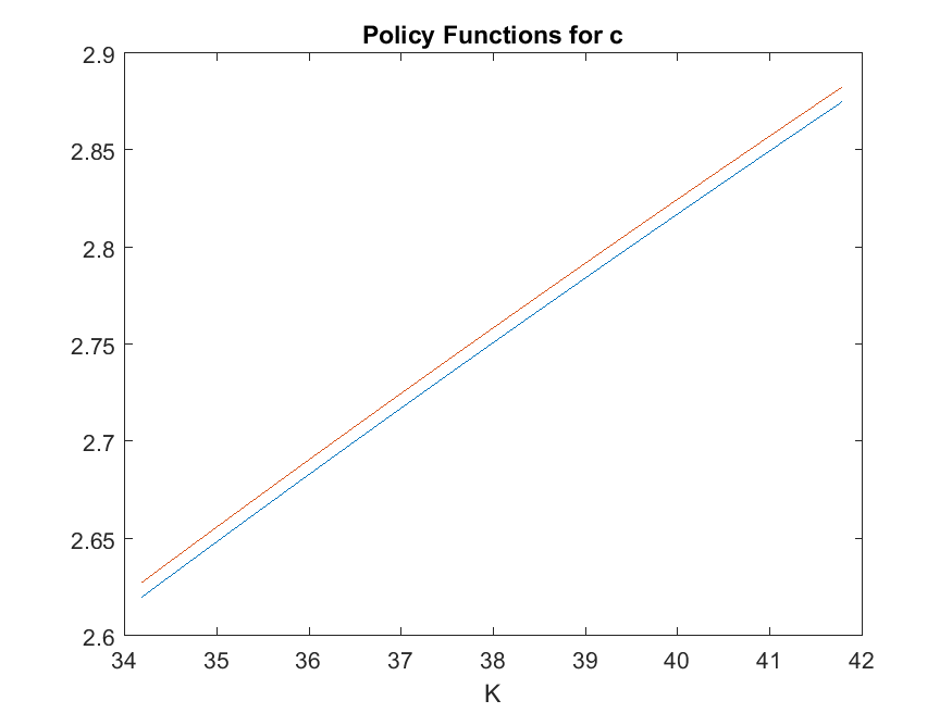
The returned IterRslt contains the converged policy and state transition functions. For example, we can plot the policy function for consumption \(c\):

>> plot(IterRslt.var_state.K, IterRslt.var_policy.c);
xlabel('K'); title('Policy Functions for c');

We can now simulate the model by inputting IterRslt into simulate_rbc:

>> SimuRslt = simulate_rbc(IterRslt);

Periods: 1000
    shock       K       c       w
        2   36.27   2.707   2.448
Elapsed time is 0.642607 seconds.

...

Periods: 10000
    shock       K       c       w
        1   36.71   2.685   2.224
Elapsed time is 0.632642 seconds.

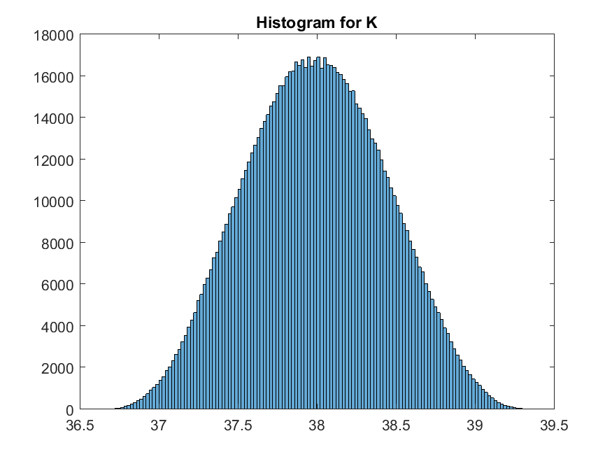
The returned SimuRslt contains a panel of simulated paths with num_samples and num_periods specified in the mod file. For example, we can plot the histogram of state variable \(K\):

>> histogram(SimuRslt.K); title('Histogram for K');

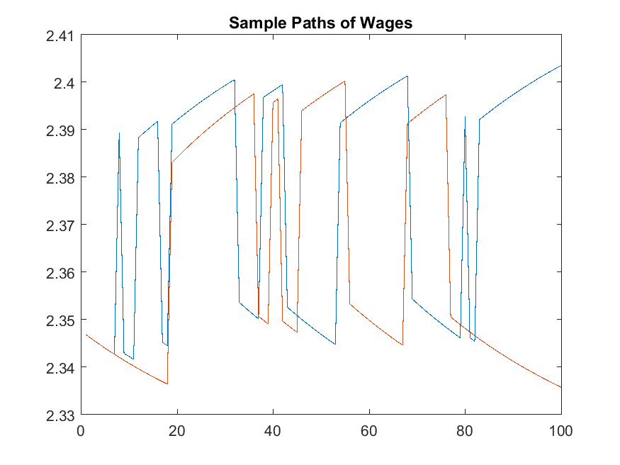
Or we can plot the first two sample paths of wages for the first 100 periods:

>> plot(SimuRslt.w(1:2,1:100)'); title('Sample Paths of Wages');

The iter and simulate files can be reused by passing parameters to be overwritten in a struct. For example,

>> options.sigma = 1.5 % overwrite sigma
options.z = [0.95,1.05] % making the shock larger
IterRslt = iter_rbc(options);
SimuRslt = simulate_rbc(IterRslt,options);

Part of the toolbox options can also be overwritten by including them in the struct. See Options.

Dissecting the gmod File

We now look into each line of rbc.gmod and describe the usage.

% Parameters
parameters beta sigma alpha delta;
beta  = 0.99;		% discount factor
sigma = 2.0;		% CRRA coefficient
alpha = 0.36;		% capital share
delta = 0.025;		% depreciation rate

A line starting with keyword parameters declares parameters. Parameters are variables used in the model block that are invariant across states or over time. Matlab-style inline comments can be used following a “%”.

% Exogenous States
var_shock z;
shock_num = 2;
z_low = 0.99; z_high = 1.01;
Pr_ll = 0.9;  Pr_hh  = 0.9;
z = [z_low,z_high];
shock_trans = [
  Pr_ll, 1-Pr_ll
  1-Pr_hh, Pr_hh
  ];

Exogenous states such as the productivity shock in the RBC model should be declared following keyword var_shock. The number of states should be specified in variable shock_num. The Markov transition matrix should be specified in variable shock_trans. Notice that any Matlab expressions such as z_low = 0.99 can be evaluated outside the model block.

For multi-dimension exogenous states, shock_num needs to be specified as the number of discretze points in the Cartesian set across all dimensions. shock_trans should be specified as the full transition matrix accordingly. Matlab functions ndgrid and kron can be used to construct the Cartesian set and the full transition matrix.

If an exogenous state follows a continuous process such as AR(1), specify the state to be an endogenous state instead in var_state, and discretize the innovation.

% Endogenous States
var_state K;
Kss  = (alpha/(1/beta - 1 + delta))^(1/(1-alpha));
KPts = 101;
KMin = Kss*0.9;
KMax = Kss*1.1;
K    = linspace(KMin,KMax,KPts);

Endogenous states such as capital in the RBC model should be declared following keyword var_state. Then the discretized grid for each state should be specified (e.g., K = linspace(KMin,KMax,KPts); in the example). Notice that any Matlab expressions (such as function linspace here) can be evaluated.

The discretized grid will be used in fixed-grid function approximation procedures such as splines and linear interpolations. For adaptive grid methods, only the range of the grid will be used.

% Interp
var_interp c_interp;
initial c_interp z.*K.^alpha+(1-delta)*K;
% Time iterations update
c_interp = c;

The time iteration procedure requires taking the state transition functions (here, implicitly defined in \(c_{t+1}(z,K)\)) as given when evaluating the system of equations. These state transition functions are declared following keyword var_interp. They are named var_interp since they are usually evaluated with some function approximation procedure such as interpolation in evaluating the system of equations.

Each of the transition functions needs to be initialized following keyword initial. Here \(c_{t+1}(z,K)\) is initialized as \(zK^{\alpha} + (1-\delta)K\) which means that consumers just consumer all resources that include output and non-depreciated capital. This initialization basically requests the toolbox to find the equilibrium that corresponds to the limit of a finite-horizon economy taking the number of horizons to infinity, of which \(c_{t+1}\) is initialized to be the last-period solution. Notice that the Matlab “dot” operator (.*) works in the line following initial, and relevant tensors are formed automatically.

In general, it is crucial to form a good initial guess on the transition functions to make the policy iteration method work. Starting with a last-period problem is shown to deliver both good theoretical properties and robust numerical computations (Cao, 2018). See Mendoza (2010) for an example on how to define a more complex last-period problem that may require solving a different system of equations, through a model_init block.

The update of the transition function after a time iteration step needs to be specified such as c_interp = c;. The update can use any variables returned as part of the solution to the system in the current time iteration step. For example, here c_interp = c; means that the c_interp variable is updated with c after a time iteration, where c is one of the policy variables solved by the system of equations, specified in the gmod file as below.

% Endogenous variables as unknowns of equations
var_policy c K_next;
inbound c       0 z.*K.^alpha+(1-delta)*K;
inbound K_next  0 z.*K.^alpha+(1-delta)*K;

All policy variables that enter the equations as unknowns are declared following keyword var_policy. For each of these variables, the bounds for where the equation solver searches the solution should be specified following keyword inbound. For variables of which the bounds cannot be determined ex-ante, specify tight bounds for them and use an adaptive option so the solver adjusts bounds automatically when it cannot find solutions and adapt bounds across time iterations. See var_policy in Variable declaration.

% Other endogenous variables
var_aux w;

Some policy variables can be evaluated as simple functions of states and other policy variables, so they do not have to be directly included in the system of equations. For example wage is determined by the marginal product of labor and can be evaluated according to \(w=(1-\alpha)zK^{\alpha}\). These policy variables can be declared following keyword var_aux.

model;
  % Budget constraints
  u_prime = c^(-sigma);
  kret_next' = z'*alpha*K_next^(alpha-1) + 1-delta;
  
  % Evaluate the interpolation object to get future consumption
  c_future' = c_interp'(K_next);
  u_prime_future' = c_future'^(-sigma);
  
  % Calculate residual of the equation
  euler_residual = 1 - beta*GDSGE_EXPECT{u_prime_future'*kret_next'}/u_prime;
  market_clear = z*K^alpha + (1-delta)*K - c - K_next;
  
  % Calcualte other endogenous variables
  w = z*(1-alpha)*K^alpha;
  
  equations;
    euler_residual;
    market_clear;
  end;
end;

The model;—end; block defines the system of equations for each collocation point of endogenous states and exogenous states. For the current example, it simply defines the system of equations for each collocation point \((z,K)\).

The equations should be eventually specified in the equation;—end; block, in which each line corresponds to one equation in the system. Any calculations in order to evaluate these equations are included in the model block preceding the equations block. Notice the whole model block is parsed into C++, so all evaluations should be scalar-based: Matlab functions such as .* operator cannot be used. Nevertheless, the model block supports simple control-flow blocks in Matlab-style syntax, such as if-elseif-else-end block and for-end block.

A variable followed by a prime (’) indicates that the variable is a vector of length shock_num. For example,

  kret_next' = z'*alpha*K_next^(alpha-1) + 1-delta;

means that

kret_next(1) = z(1)*alpha*K_next^(alpha-1) + 1-delta
kret_next(2) = z(2)*alpha*K_next^(alpha-1) + 1-delta

A var_shock (here z), when used followed by a prime (‘), corresponds to the vector of the variable across all possible exogenous states, and thus can be used to construct other vector variables. Notice when a var_shock is used not followed by a prime, it corresponds to the exogenous state at the current collocation point, e.g., z in

  market_clear = z*K^alpha + (1-delta)*K - c - K_next;

Any var_interp declared before can be used as a function in the model block. For example,

  c_future' = c_interp'(K_next);

means calculating \(c_{t+1}\) based on the state transition function implied by c_interp, at the next-period endogenous state K_next (which is a current policy variable). Where are the next-period exogenous states? These are taken care of by the prime (’) operator following c_interp, which means that it is evaluating at each realization of the future exogenous states, and returning a vector of length shock_num. Accordingly, the left hand side variable should be declared as a vector, i.e., a variable followed by a prime (‘).

The model block can use several built-in functions for reduction operations. For example, the GDSGE_EXPECT{} used in

  euler_residual = 1 - beta*GDSGE_EXPECT{u_prime_future'*kret_next'}/u_prime;

is to calculate the conditional expectation of the object defined inside the curly braces, conditional on the current exogenous state, using the default Markov transition matrix shock_trans. Obviously, this function is meaningful only if it takes as argument the realizations of variables across future exogenous states, which are defined as vector variables followed by prime (‘).

This operator can also take a different transition matrix than shock_trans, which is used as GDSGE_EXPECT{*|alternative_shock_trans}. This can be used to solve models with heterogeneous beliefs. See example Cao (2018).

Two other reduction operations GDSGE_MAX{} and GDSGE_MIN{} are defined, which are to take the maximum and the minimum of objects inside the curly braces, respectively. See Built-in functions.

simulate;
  num_periods = 10000;
  num_samples = 6;
  initial K Kss;
  initial shock 1;
  var_simu c K w;
  K' = K_next;
end;

The simulate block defines how the file for Monte Carlo simulations should be generated. It should define the initial endogenous state following keyword initial. initial K Kss; in the example sets the endogenous state \(K\) to Kss defined before.

The simulate block should define the initial exogenous state index following keyword initial shock. It should define the variables to be recorded following var_simu. It should define the transition for each state variable. In the example, K'=K_next; defines that the next period endogenous state \(K\) should be assigned to K_next which is one of the var_policy solved as part of the system. Notice the prime operator (’) following K indicates that the line is to specify the transition of an endogenous state variable in the simulation, which has a different meaning than the prime operator (’) used in the model block. Nevertheless, the prime operators (’) in both usages are associated with the transition to the future state, and thus motivate such designs.

The simulate block can also overwrite num_periods (default 1000) and num_samples (default 1).

Comparisons with Dynare

Dynare is a MATLAB/Octave-based toolbox to solve a wide range of macroeconomic models including DSGE, OLG, perfect foresight and more. Dynare is specialized in solving DSGE models with local perturbation methods, whereas GDSGE is designed to obtain global solutions.

As perhaps noted by experienced Dynare users, GDSGE follows the many design features of Dynare. However, due to the nature of global solutions, the gmod code file requires more user input which makes it a bit more lengthy than the Dynare mod file. In particular, the global solution requires the explicit definition of state variables and the STFPI algorithm requires the update rule for the policy functions, neither of which are needed by Dynare.

For bridging Dynare users to GDSGE, below is a line-by-line walkthrough to convert the Dynare mod file into the GDSGE gmod file, for the simple RBC model listed here. Note some of the parameter values and code organizations have been slightly modified from the original gmod file, so as to enable the comparison. The updated gmod file and and the corresponding Dynare mod file can be downloaded here: rbc_simple.gmod; rbc_simple.mod

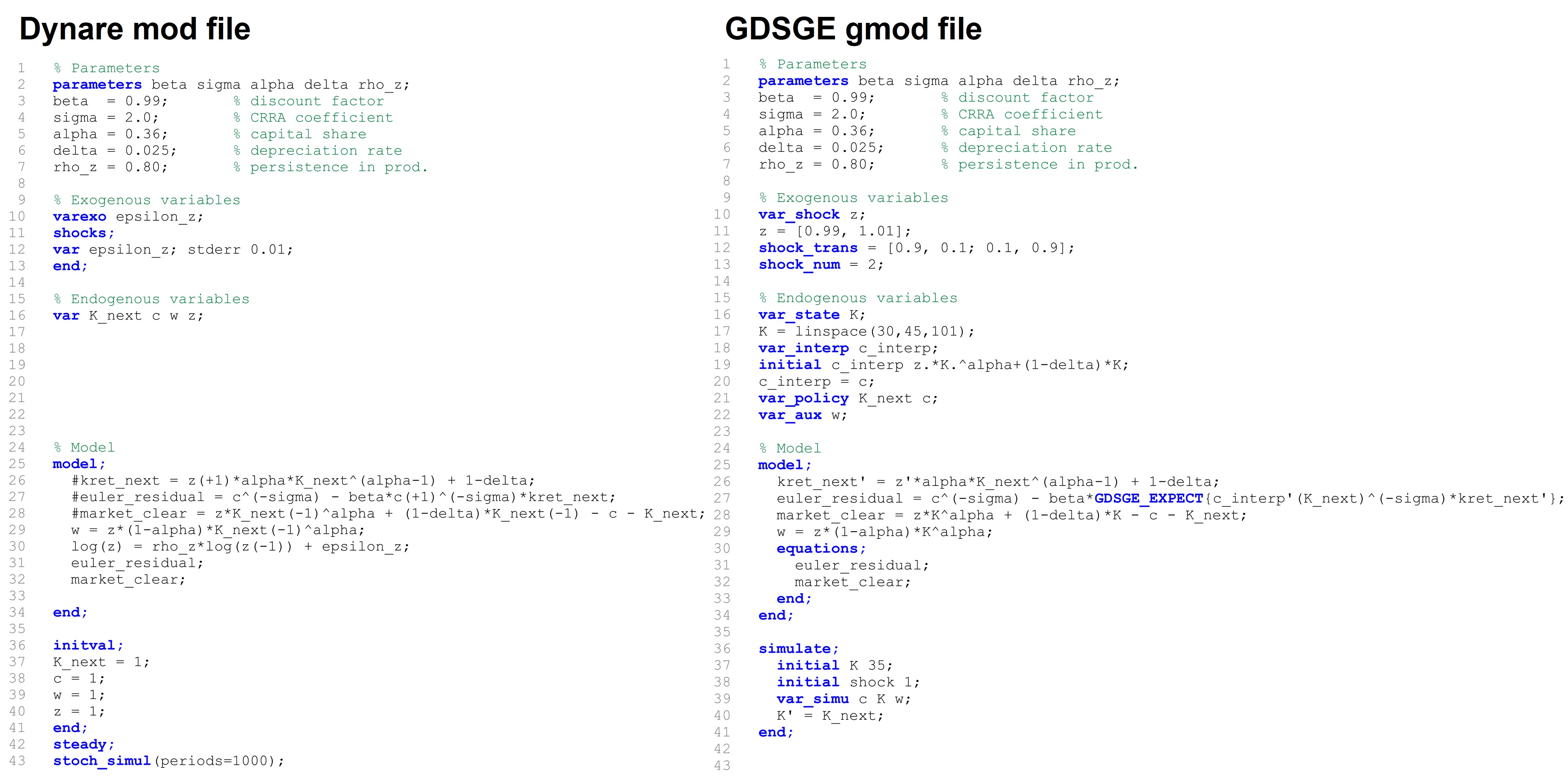
In more details:

• Line 2-Line 7: definitions of parameters are exactly the same.

• Line 10-Line 13: the Dynare mod file defines the exogenous shocks by specifying it to be a varexo and a var in the shocks block, whereas in the GDSGE gmod file the shock needs to be discretized into a Markov chain, with the number of discrete values specified in shock_num and the Markov transition matrix specified in shock_trans.

• Line 15-Line 22: the Dynare mod file defines all endogenous variables, regardless of them being state or jump variables, as var. The GDSGE gmod file needs to breakdown those variables into different blocks:

  (1) var_state: state variables (here, capital stock \(K\)), with the grid of each state variables explicitly specified (here, by Line 17).

  (2) var_interp: a subset of policy variables that are necessary to evaluate the inter-temporal equilibrium conditions, here, consumption \(c\) in order to evaluate the Euler equations, renamed to be c_interp; the initial value and the update rule for each of the var_interp also need to be specified (here, by Line 19 and 20).

  (3) var_policy: policy variables that directly enter the system of equations as unknowns.

  (4) var_aux: policy variables that are simple functions of state variables and other policy variables and can be directly evaluated.

• Line 24-Line 34: the model block. In the Dynare model block, all intermediate variables are defined with a prefix # and all other statements define an equation of the equilibrium systems. In the GDSGE model block, instead, each line represents an assignment, and the system of equations needs to be defined in the equations block explicitly.

• Line 36-Line 43: the model solver. Dynare requires the specification of the initial value of steady state variables in the initval block, followed by steady and stoch_simul commands to solve the steady state and the local solutions. GDSGE does not require the input of the initial values in most cases; GDSGE solves an equilibrium system at each collocation point to get the global solution, beyond the steady state. A simulate block needs to be specified instead, to specify the initial value and the transition of state variables, which generates codes for Monte-Carlo simulations.

What’s Next?

The current example demonstrates the basic usage of the toolbox. The global solutions obtained by GDSGE can be used to analyze models with highly nonlinear and state-dependent dynamics, such as models with an occasionally binding borrowing constraint or interest rate zero lower bound. An alternative method to analyze the nonlinear solutions is the piecewise local solution method, popularized by the method and toolbox OccBin (Guerrieri and Iacoviello, 2015).

We provide an example of an model with an occasionally binding interest rate zero lower bound that can be solved by both OccBin and GDSGE, to further introduce GDSGE to users who are familiar with Dynare and OccBin. See A Simple Model with an Interest Rate ZLB.

You can also proceed to an extension of RBC model with investment irreversibility that requires a global method, or to Heaton and Lucas (1996) which is the leading example in the toolbox paper.

Or you can proceed to Toolbox API.