Barro et al. (2017): Safe Assets with Rare Disasters

The model studies the creation of safe assets (risk-free bonds) between two agents with different risk aversion levels, in an endowment economy with rare disaster shocks. The model serves as an example to demonstrate how the toolbox can accommodate general recursive preferences such as Epstein and Zin (1989) - Weil (1990), which is a common preference specification in the asset pricing and macro finance literature. The example also demonstrates that the solution method can handle ill-behaved equilibrium systems robustly: in the context of Barro et al. (2017), when the risk aversion level is set very high (e.g., with coefficient of relative risk aversion up to 100), the traditional nested fixed point solution method becomes unstable, since agents’ portfolio choice becomes very sensitive to the pricing function. Nevertheless, the toolbox, which solves the equilibrium as one single system of equations, can handle such parameterization fairly easily and uncovers novel theoretical results.

The Model

There are two groups of agents, \(i=1,2\) in the economy. Agents have an Epstein and Zin (1989) - Weil (1990) utility function. The coefficients of risk aversion satisfy \(\gamma_{2}\geq\gamma_{1}>0\), i.e., agent 1 is less risk-averse than agent 2. The other parameters between these two groups are the same. There is a replacement rate \(\upsilon\) at which each type of agents move to a state that has a chance of \(\mu_{i}\) of switching into type \(i\). Taking the potential type shifting into consideration, their utility function can be written as

\[U_{i,t}=\left\{ \frac{\rho+\upsilon}{1+\rho}C_{i,t}^{1-\theta}+\frac{1-\upsilon}{1+\rho}\left[\mathbb{E}_{t}\left(U_{i,t+1}^{1-\gamma_{i}}\right)\right]^{\frac{1-\theta}{1-\gamma_{i}}}\right\} ^{1/\left(1-\theta\right)}.\label{eq:utility SafeAssets}\]

In this economy, there is a Lucas tree generating consumption good \(Y_{t}\) in period \(t\) consumed by both agents. \(Y_{t}\) is subject to identically and independently distributed rare-disaster shocks. With probability \(1-p\), \(Y_{t}\) grows by the factor \(1+g\); with a small probability \(p\), \(Y_{t}\) grows by the factor \(\left(1+g\right)\left(1-b\right)\). Thus the expected growth rate of \(Y_{t}\) in each period is \(g^{*}\approx g-pb.\) Denote agent \(i\)’s holding of the tree as \(K_{it}\). The supply of the Lucas tree is normalized to one, and denote its price as \(P_{t}\). The gross return of holding equity is \(R_{t}^{e}=\frac{Y_{t}+P_{t}}{P_{t-1}}\). Agents also trade a risk-free bond, \(B_{it}\), whose net supply is zero, and the gross interest rate is \(R_{t}^{f}\).

Denote the beginning-of-period wealth of agent \(i\) by \(A_{it}\). Each agent’s budget constraint is

\[C_{it}+P_{t}K_{it}+B_{it}=A_{it}.\]

Considering the type shifting shock, the law of motion of \(A_{it}\) is

\[A_{it}=\left(Y_{t}+P_{t}\right)\left[K_{it-1}-\upsilon\left(K_{it-1}-\mu_{i}\right)\right]+\left(1-\upsilon\right)R_{t}^{f}B_{it-1}.\]

As in Cao (2018, Appendix C.3, Extension 3), we can normalize the utility \(U_{it}\) and consumption \(C_{it}\) by \(A_{it}\) and write recursive utility as follows:

(4)\[u_{it}^{1-\theta}=\frac{\rho+\upsilon}{1+\rho}c_{i,t}^{1-\theta}+\frac{1-\upsilon}{1+\rho}\left(1-c_{it}\right)^{1-\theta}\left(\mathbb{E}_{t}\left[\left(R_{i,t+1}u_{it+1}\right)^{1-\gamma_{i}}\right]\right)^{\frac{1-\theta}{1-\gamma_{i}}},\]

in which \(u_{it}=U_{it}/A_{it}\), \(c_{it}=C_{it}/A_{it}\), and

\[R_{i,t+1}=x_{it}R_{t+1}^{e}+\left(1-x_{it}\right)R_{t+1}^{f}\]

is the average return of agent \(i\)’s portfolio, and

\[x_{it}=\frac{P_{t}K_{it}}{P_{t}K_{it}+B_{it}}\]

is the equity share of agent \(i\)’s portfolio holding. The FOCs for consumption and portfolio choices are

(5)\[\left(\rho+\upsilon\right)c_{i,t}^{-\theta}=\left(1-\upsilon\right)\left(1-c_{it}\right)^{-\theta}\left[\mathbb{E}_{t}\left(R_{i,t+1}u_{it+1}\right)^{1-\gamma_{i}}\right]^{\frac{1-\theta}{1-\gamma_{i}}},\]

and

(6)\[\mathbb{E}_{t}\left[\frac{\left(R_{t+1}^{e}-R_{t+1}^{f}\right)u_{it+1}}{\left(R_{i,t+1}u_{it+1}\right)^{\gamma_{i}}}\right]=0.\]

The choices of \(c_{it}\) and \(x_{it}\) are identical across agents of the same type \(i\), and the portfolio choices of agent \(i\) are

\[\begin{split}K_{it} & =x_{it}\left(1-c_{it}\right)\left(1+p_{t}\right)/p_{t}\omega_{it},\\ b_{it} & =\left(1-x_{it}\right)\left(1-c_{it}\right)\left(1+p_{t}\right)\omega_{it}.\end{split}\]

In equilibrium, prices are determined such that markets clear:

(7)\[C_{1t}+C_{2t} =Y_{t},\]

(8)\[K_{1t}+K_{2t} =1,\]

(9)\[B_{1t}+B_{2t} =0.\]

To achieve stationarity, we normalize \(\left\{ B_{it},P_{t}\right\}\) variables by \(Y_{t}\). We define the wealth share of agent \(i\) as

(10)\[\omega_{it}=K_{it-1}-\upsilon\left(K_{it-1}-\mu_{i}\right)+\frac{\left(1-\upsilon\right)R_{t}^{f}b_{it-1}}{\left(1+p_{t}\right)\left(1+g_{t}\right)}.\]

We see that given the market clearing conditions (8) and (9),

\[\omega_{1t}+\omega_{2t}=1,\:\forall t.\]

For much of the analysis in Barro et al. (2017), the intertemporal elasticity of substitution \(\theta\) is set at \(1\). In this case, agents consume a constant share of their wealth, and equation (5) is replaced by

\[c_{it}=\frac{\rho+\upsilon}{1+\rho}.\]

Using this relationship for \(i=1,2\), and use the market clearing conditions (7), (8) and (9), we have

\[p_{t}=\frac{1-\upsilon}{\rho+\upsilon}.\]

The utility function (4) is replaced by

\[\begin{split}\log u_{it}= & \frac{\rho+\upsilon}{1+\rho}\log c_{it}+\frac{1-\upsilon}{1+\rho}\log\left(1-c_{it}\right)\\ & +\frac{1-\upsilon}{1+\rho}\frac{1}{1-\gamma_{i}}\log\left[\mathbb{E}_{t}\left(R_{i,t+1}u_{it+1}\right)^{1-\gamma_{i}}\right].\end{split}\]

The state variable is \(\omega_{1t}\). The unknowns are \(\left\{ x_{1t},x_{2t},R_{t}^{f},\omega_{it+1}\left(z_{t+1}\right)\right\}\). We have 4 equations: (6) for \(i=1,2\), the market clearing condition for bond (9) and the consistency equation (10) to solve the unknowns.

The gmod File

The model is solved with the following safe_assets.gmod file

% Parameters
parameters rho nu mu gamma1 gamma2;
period_length=0.25;         % a quarter
rho = 0.02*period_length;   % time preference
nu = 0.02*period_length;    % replacement rate
mu = 0.5;                   % population share of agent 1
P = 1-exp(-.04*period_length);   % disaster probability
B = -log(1-.32);            % disaster size
g = 0.025*period_length;    % growth rate
gamma1 = 3.1;
gamma2 = 50;

% Shocks
var_shock yn;
shock_num = 2;
shock_trans = [1-P,P;
               1-P,P];
yn = exp([g,g-B]);

% States
var_state omega1;
Ngrid = 501;
omega1 = [linspace(0,0.03,200),linspace(0.031,0.94,100),linspace(0.942,0.995,Ngrid-300)];

p = (1-nu)/(rho+nu);
pn = p;
Re_n = (1+pn)*yn/p;
% Endogenous variables, bounds, and initial values
var_policy shr_x1 Rf omega1n[2]
inbound shr_x1 0 1;             % agent 1's equity share
inbound Rf Re_n(2) Re_n(1);     % risk-free rate
inbound omega1n 0 1.02;         % state next period

% Other equilibrium variables
var_aux x1 x2 K1 b1 c1 c2 log_u1 log_u2 expectedRe;

% Implicit state transition functions
var_interp log_u1future log_u2future;
log_u1future = log_u1;
log_u2future = log_u2;
initial log_u1future (rho+nu)/(1+rho)*log((rho+nu)/(1+rho)) + (1-nu)/(1+rho)*log((1-nu)/(1+rho));
initial log_u2future (rho+nu)/(1+rho)*log((rho+nu)/(1+rho)) + (1-nu)/(1+rho)*log((1-nu)/(1+rho));

model;
  c1 = (rho+nu)/(1+rho);
  c2 = (rho+nu)/(1+rho);
  p = (1-nu)/(rho+nu);
  pn = p;

  log_u1n' = log_u1future'(omega1n');
  log_u2n' = log_u2future'(omega1n');
  u1n' = exp(log_u1n');
  u2n' = exp(log_u2n');

  Re_n' = (1+pn)*yn'/p;
  x1 = shr_x1*(Rf/(Rf - Re_n(2)));
 
  % Market clearing for bonds:
  b1 = omega1*(1-x1)*(1-c1)*(1+p);
  b2 = -b1;
  x2 = 1 - b2/((1-omega1)*(1-c2)*(1+p));
  K1 = x1*(1-c1)*omega1*(1+p)/p;
  K2 = x2*(1-c2)*(1-omega1)*(1+p)/p;

  R1n' = x1*Re_n' + (1-x1)*Rf;
  R2n' = x2*Re_n' + (1-x2)*Rf;

  % Agent 1's FOC wrt equity share:
  eq1 = GDSGE_EXPECT{Re_n'*u1n'^(1-gamma1)*R1n'^(-gamma1)} / GDSGE_EXPECT{Rf*u1n'^(1-gamma1)*R1n'^(-gamma1)} - 1;

  % Agent 2's FOC wrt equity share:
  log_u2n_R2n_gamma' = log_u2n'*(1-gamma2) - log(R2n')*gamma2;
  min_log_u2n_R2n_gamma = GDSGE_MIN{log_u2n_R2n_gamma'};
  log_u2n_R2n_gamma_shifted' = log_u2n_R2n_gamma' - min_log_u2n_R2n_gamma;
  eq2 = GDSGE_EXPECT{Re_n'*exp(log_u2n_R2n_gamma_shifted')} / GDSGE_EXPECT{Rf*exp(log_u2n_R2n_gamma_shifted')} - 1;

  % Consistency for omega:
  omega_future_consis' = K1 - nu*(K1-mu) + (1-nu)*Rf*b1/(yn'*(1+pn)) - omega1n';

  % Update the utility functions:
  ucons1 = ((rho+nu)/(1+rho))*log(c1) + ((1-nu)/(1+rho))*log(1-c1);
  ucons2 = ((rho+nu)/(1+rho))*log(c2) + ((1-nu)/(1+rho))*log(1-c2);
  log_u1 = ucons1 + (1-nu)/(1+rho)/(1-gamma1)*log(GDSGE_EXPECT{(R1n'*u1n')^(1-gamma1)});        
  log_u2 = ucons2 + (1-nu)/(1+rho)/(1-gamma2)*( log(GDSGE_EXPECT{R2n'*exp(log_u2n_R2n_gamma_shifted')}) + min_log_u2n_R2n_gamma );

  expectedRe = GDSGE_EXPECT{Re_n'};
       
  equations;
    eq1;
    eq2;
    omega_future_consis';
  end;
end;

simulate;
  num_periods = 10000;
  num_samples = 50;
  initial omega1 .67;
  initial shock 1;
  
  var_simu Rf K1 b1 expectedRe;

  omega1' = omega1n';
end;

There is not too much new about the usage of the toolbox if you already saw examples Heaton and Lucas (1996) and Guvenen (2009). There are some transformations worth mentioning which facilitate solving the model.

  % Agent 2's FOC wrt equity share:
  log_u2n_R2n_gamma' = log_u2n'*(1-gamma2) - log(R2n')*gamma2;
  min_log_u2n_R2n_gamma = GDSGE_MIN{log_u2n_R2n_gamma'};
  log_u2n_R2n_gamma_shifted' = log_u2n_R2n_gamma' - min_log_u2n_R2n_gamma;
  eq2 = GDSGE_EXPECT{Re_n'*exp(log_u2n_R2n_gamma_shifted')} / GDSGE_EXPECT{Rf*exp(log_u2n_R2n_gamma_shifted')} - 1;

These lines describe how to calculate the Euler Equation residual

\[\mathbb{E}_{t}\left[\frac{\left(R_{t+1}^{e}-R_{t+1}^{f}\right)u_{it+1}}{\left(R_{i,t+1}u_{it+1}\right)^{\gamma_{i}}}\right]=0\]

when the CRRA coefficient \(\gamma_2\) is very large: by tracking and calculating the log level of utility instead of the level of utility. This procedure proves to be essential in solving models with \(\gamma_2\) very high, as \(u\) can easily fall below the smallest number permitted by double precision.

As in previous examples, we can inspect the policy functions and ergodic sets after solving policy iterations and simulations. Here, we focus on how to construct generalized impulse responses using the model simulations. Since the equilibrium concept involves an ergodic distribution of state, instead of a deterministic steady state, the proper concepts of impulse responses are sampling responses from the ergodic set, and taking their averages and standard deviations. The sampling procedure can be done on a sub-population of the ergodic set, generating conditional impulse responses which will be of particular interests since the non-linear models may feature different dynamics starting from different part of the state space.

The procedure for constructing generalized impulse responses goes as follows:

1. Simulate an ergodic set, which can be done by simulating one or multiple samples for a long-period of time, according to the Ergodic theorem.

2. Replicate the ergodic set to get two identical sets. For one of the two, turn the shock to “on”. The exact procedure depends on the model. In the current example, “on” corresponds to the rare diaster state. For the other set, keep the shock unchanged.

3. Simulate the two sets, keeping the transitions of the exogenous shocks on. This procedure essentially captures the effect of the switching of the shock in the initial period on subsequent dynamics.

4. Calculate the mean and standard deviation of the differences between simulated time series of the two sets. These arrive at the mean impulse responses and the standard deviations. Again, the above procedure can be conditional on a sub-population of the ergodic set so as to compute conditional impulse responses starting from states with certain properties of interests.

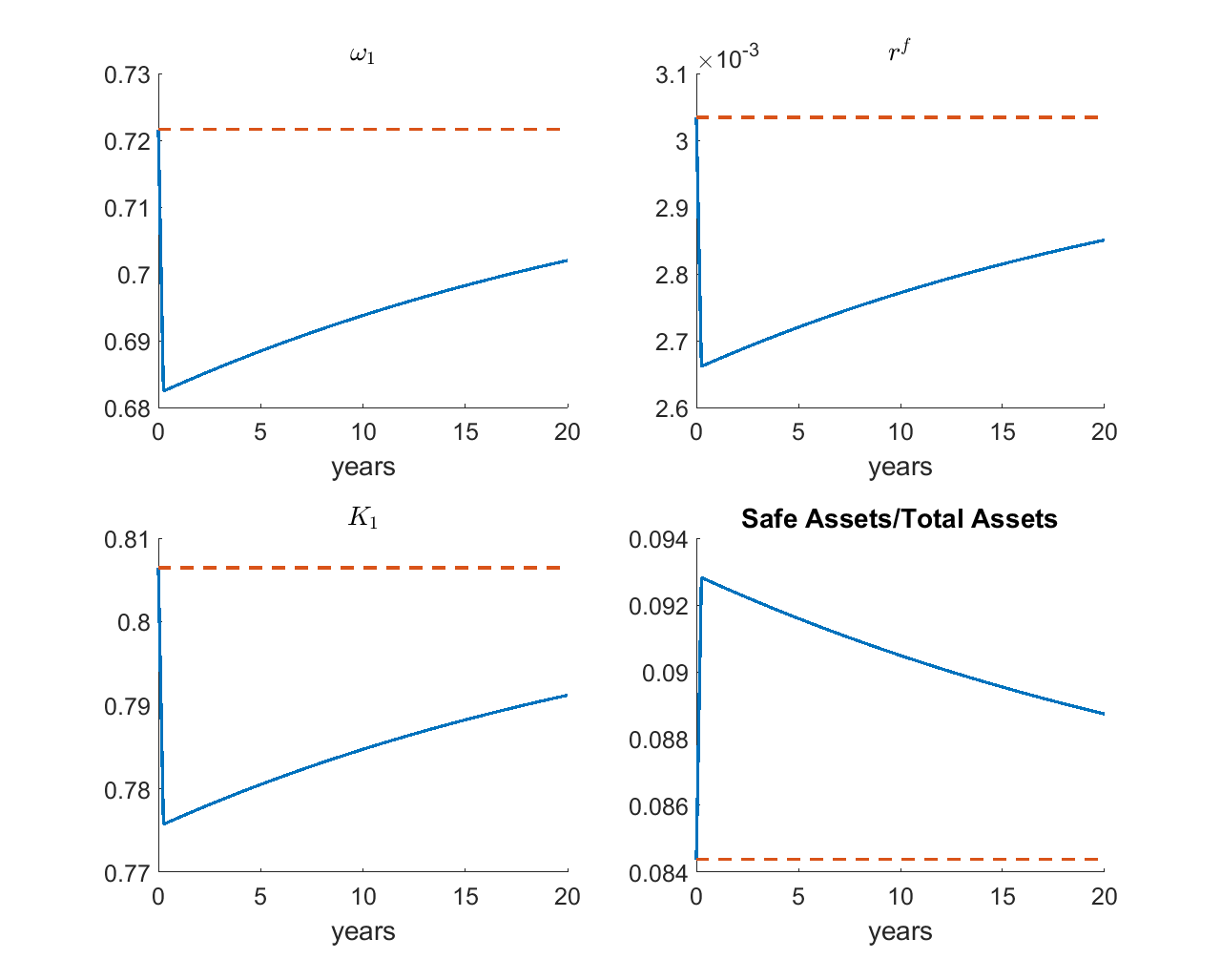
The figure plots the impulse responses after a one-time disaster using the baseline parameters in Barro et al. (2017). (For annual data, \(\rho=0.02\), \(\upsilon=0.02\), \(\mu=0.5\), \(\gamma_{1}=3.3\), and \(\gamma_{2}=5.6\). Growth rate in normal times is \(0.025\). Rare disaster happens with probability 4%, and once it happens, productivity drops by 32%. The model period is one quarter.) As shown in the figure, the rare disaster shock redistributes wealth from the less risk averse agents (Agent 1) to the more risk averse agents (Agent 2). This leads to more demand for safe asset, and a higher equilibrium quantity and price (lower interest rate) of the safe asset.

A final remark is on the price of safe assets, which exhibits non-monotonicity as the risk aversion of Agent 2 \(\gamma_2\) increases, as shown in the figure below. This non-monotonicity is usually overlooked in the literature and uncovered by our solution method that can solve models with high \(\gamma_2\) robustly and accurately.

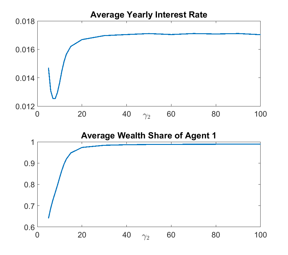
The mechanism behind the non-monotonicity can be understood by looking at two opposing forces. First, as \(\gamma_{2}\) gets larger, agent 2 becomes more risk-averse, and demand for more of the safe asset (bond). This pushes down \(\bar{R}^{f}\). Second, an increase in \(\gamma_{2}\) also leads agent \(1\) to borrow more and become more leveraged. Since the return of equity is higher than bond, the average wealth share of agent 1, \(\omega_{1}\) becomes larger. Larger \(\omega_{1}\) leads to more relative supply of safe asset and pushes up \(\bar{R}^{f}\). Whether \(\bar{R}^{f}\) decreases or increases in \(\gamma_{2}\) depends on which force dominates. The figure shows that when \(\gamma_{2}\) is below \(8\) the first force dominates and \(\bar{R}^{f}\) is decreasing in \(\gamma_{2}\) as assumed in Barro et al. (2017). However, when \(\gamma_{2}\) is larger than \(8\), the second force dominates and \(\bar{R}^{f}\) is increasing in \(\gamma_{2}\). When \(\gamma_{2}\) is larger than 20, \(\bar{R}^{f}\) is not responsive to \(\gamma_{2}\), since the wealth distribution \(\omega_{1}\) is almost degenerated to its upper limit.

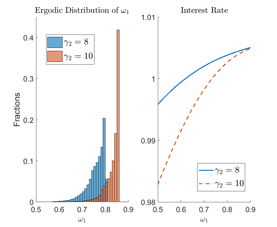
The figure below provides a comparison of two cases: \(\gamma_{2}=8\) versus \(\gamma_{2}=10\). As \(\gamma_2\) increases, the wealth share of Agent 1 tends to be larger.

What’s Next?

This example illustrates that the toolbox algorithm is especially effective to solve models where portfolio choices are sensitive to the asset price, which are traditionally considered ill-behaved problems. In Cao, Evans, and Luo (2020), we solve another model which is traditionally considered ill-behaved: a two-country DSGE model with portfolio choices in which the returns to assets are close to collinear in certain regions of the state space.

Or you can directly proceed to Toolbox API.