An RBC Model with Irreversible Investment

The standard RBC model can also be solved easily using local methods. Now we consider an extension which can only be solved properly using global methods. The model features an investment irreversibility constraint, which requires investment to be larger than a certain threshold.

The Model

We augment the simple RBC model with two additional features.

First, productivity follows a continuous AR(1) process

\[\log z_t = \rho \log z_{t-1} + \epsilon_t\]

where parameter \(\rho \in (0,1)\) is the persistence, \(\epsilon_t\) is an I.I.D. shock.

Second, when accumulating capital,

\[K_{t+1} = K_t(1-\delta) + I_t,\]

the representative firm is subject to an irreversibility constraint

\[I_t \geq \phi I_{ss},\]

where \(I_{ss}\) is the steady-state level of investment and parameter \(\phi\) corresponds to the tightness of the irreversibility constraint.

These features require us to keep track of two continuous state variables: exogenous \(z_t\) and endogenous \(K_t\). The toolbox is well designed to handle models with more than one continuous state variables like the current one.

Let \(\mu_t\) denote the Lagrange multiplier on the irreversibility constraint, the complete-markets equilibrium can be characterized by the Euler equation, the complementary-slackness condition, and the goods market clearing condition:

\[\begin{split}&c_t^{-\sigma}-\mu_t\\ &=\beta \mathbb{E}_t \left[\left ( \alpha z_{t+1} K_{t+1}^{\alpha-1}+(1-\delta)\right)c_{t+1}^{-\sigma}-(1-\delta)\mu_{t+1}\right],\\ &\\ &\mu_t (K_{t+1}-(1-\delta)K_t-\phi I_{ss}) = 0,\\ &\\ &c_t+K_{t+1} = z_t K_t^{\alpha}+(1-\delta)K_t.\end{split}\]

A recursive competitive equilibrium consists of functions: \(c(z,K), K'(z,K), \mu(z,K)\) s.t.

\[\begin{split}&c(z,K)^{-\sigma}-\mu(z,K)\\ &=\beta \mathbb{E}\left[ \left (\alpha z' [K'(z,K)]^{\alpha-1}+(1-\delta)\right)[c(z',K'(z,K))]^{-\sigma}-(1-\delta)\mu(z',K'(z,K)) \Big| z \right]\\ &\\ &\mu(z,K)(K'(z,K)-(1-\delta)K-\phi I_{ss})=0\\ &\\ &c(z,K)+K'(z,K)=zK^{\alpha} + (1-\delta)K.\end{split}\]

This recursive system can be solved using a time iteration procedure similar to the one for the standard RBC model. In the period-\(t\) time step, we take functions \(c_{t+1}(z,K),\mu_{t+1}(z,K)\) as known, and solve for \(c_t,\mu_t,K'_t\) from the system of three equations:

\[\begin{split}&c_t(z,K)^{-\sigma}-\mu_t(z,K)\\ &=\beta \mathbb{E}\left[ \left (\alpha z' [K_t'(z,K)]^{\alpha-1}+(1-\delta)\right)[c_{t+1}(z',K_t'(z,K))]^{-\sigma}-(1-\delta)\mu_{t+1}(z',K_t'(z,K))\Big| z \right]\\ &\\ &\mu_t(z,K)(K'_t(z,K)-(1-\delta)K-\phi I_{ss})=0\\ &\\ &c_t(z,K)+K'_t(z,K)=zK^{\alpha} + (1-\delta)K.\end{split}\]

We keep iterating until convergence.

The gmod File

The recursive system can now be input to the GDSGE toolbox via a mod file rbcIrr.gmod below.

% Parameters
parameters beta sigma alpha delta K_min K_max rho Imin;

beta = 0.99; % dicount factor
sigma = 2; % risk aversion
alpha = 0.36; % capital share
delta = 0.025; % depreciation rate
rho = 0.90; %persistent of productivity shocks
phi = 0.975; %investment irreversibility constraint

TolEq = 1e-6;
SaveFreq = 50;
SimuSaveFreq = 1000;
SimuPrintFreq = 1000;
NumThreads = feature('NumCores');

% Shocks
var_shock e;
shock_num = 2;
shock_trans = [1/2.0,1/2.0;1/2.0,1/2.0];
e = [-0.01,0.01]*sqrt(1-rho^2);

% Steady state
Kss = (alpha/(1/beta - 1 + delta))^(1/(1-alpha));
Iss = delta*Kss;
Imin = phi*Iss;
K_min = 0.5*Kss;
K_max = 1.5*Kss;

% States
var_state z K;
z_pts = 21;
z = linspace(0.9,1.1,z_pts);
K_pts = 201;
K = exp(linspace(log(K_min),log(K_max),K_pts));

var_interp Euler_interp muc_interp;

% Last period
var_policy_init c;
inbound_init c 1e-6 100;

var_aux_init Euler mu muc;

model_init;
  Y = z*(K^alpha);
  resid = 1 - c/(Y-Imin);
  
  mu = 1;
  muc = mu*(c^-sigma);
  Euler = (c^-sigma)*(1-delta+z*alpha*K^(alpha-1));

  equations;
     resid;		
  end;
end;

initial Euler_interp Euler;
Euler_interp = Euler;
initial muc_interp muc;
muc_interp = muc;

% Endogenous variables, bounds, and initial values
var_policy c invst mu;

inbound c 1e-6 100 adaptive(2);
inbound invst 0 50 adaptive(1.5);
inbound mu 0 2 adaptive(1.5);

% Other equilbirium variables
var_aux Y Euler K_next muc z_next[2] Inv;

model;
  %investment irreversiility constraint    
  Inv = invst + Imin;     
  K_next = Inv + (1-delta)*K;
  Y = z*(K^alpha);
  resid  = 1 - (Inv+c)/Y;
  
  %transition to z_next
  z_next' = exp(rho*log(z)+e');
  
  %interpolation of future policies 
  Euler_future' = Euler_interp'(z_next',K_next);  
  EEuler_future = GDSGE_EXPECT{Euler_future'};   
  muc_future' = muc_interp'(z_next',K_next);
  Emuc_future = GDSGE_EXPECT{muc_future'};
  
  Euler = (c^-sigma)*(1-delta+z*alpha*K^(alpha-1));
  muc = mu*(c^-sigma);
 
  % First order conditions for firms  
  foc = 1-mu - (beta*EEuler_future-beta*(1-delta)*Emuc_future)/(c^-sigma);  
  comp_slack = mu*invst;

  equations;
      foc;
      resid;
      comp_slack; 
  end;
end;

simulate;
  num_periods = 15000;
  num_samples = 100;
  
  initial K Kss;
  initial z 1;
  initial shock 2;
  
  var_simu z K Y c Inv;
  K' = K_next;
  z' = z_next';
end;

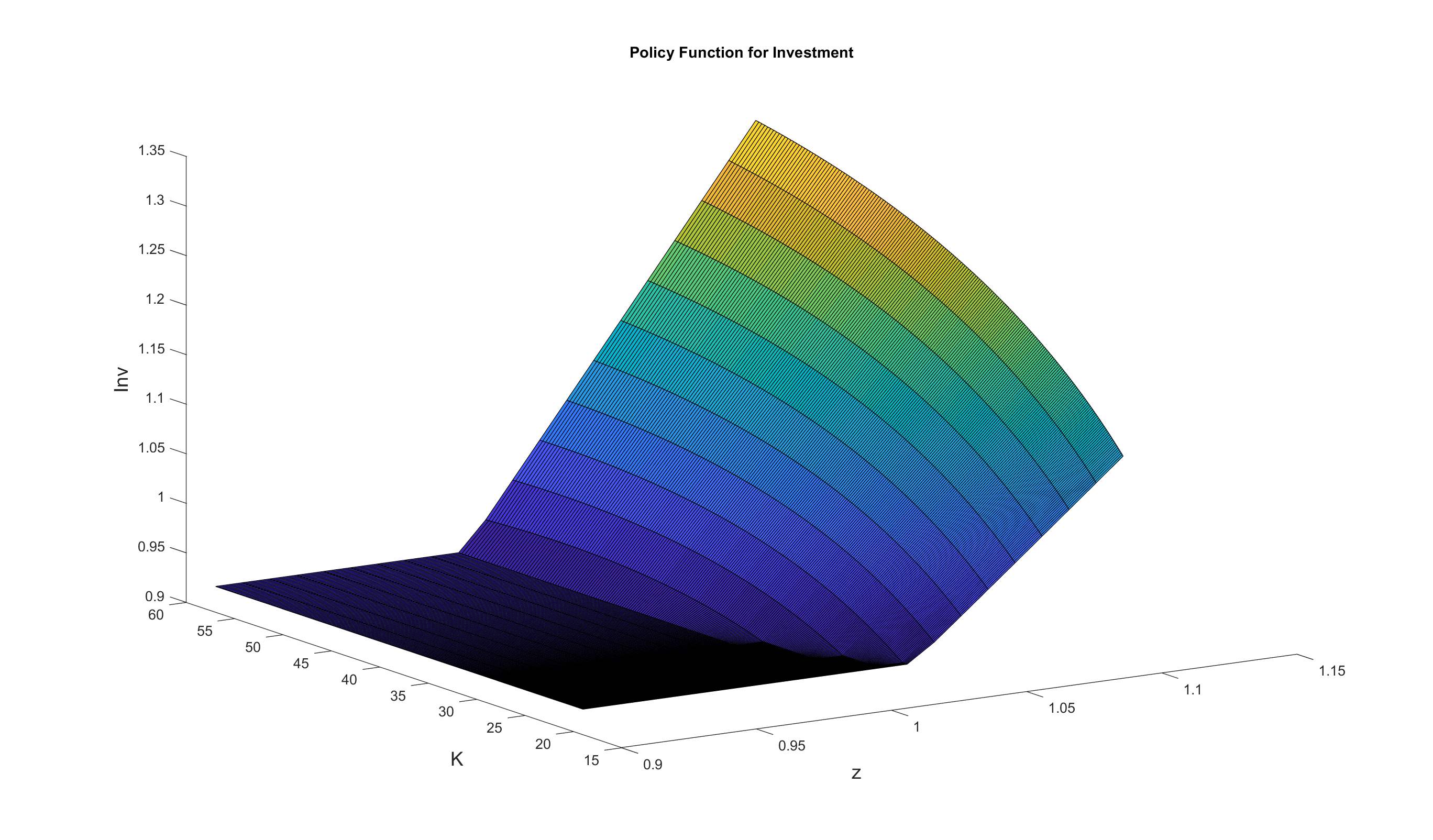
The toolbox solves the model and produces the policy functions. The following figure displays the investment policy function \(I(z,K)\). The investment irreversibility constraint tends to bind when \(K\) is low or \(z\) is low.

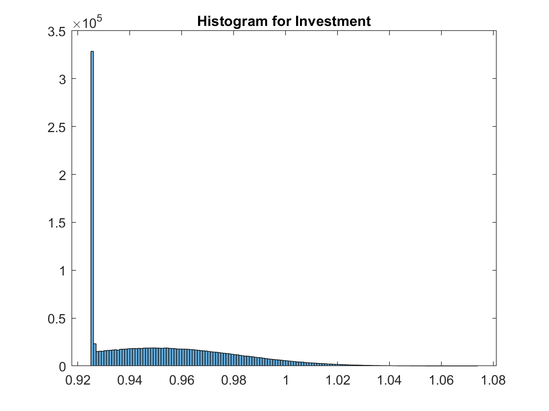
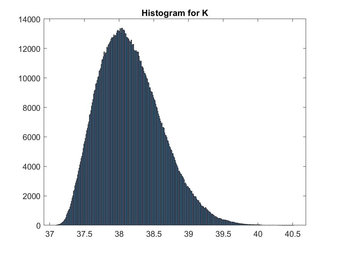
We then use the policy functions to simulate the model. The following figures show the long run distributions of investment and capital. The investment irreversibility constraint binds around 20% of the times. The distribution of capital is asymmetric and skewed towards lower levels of capital. It is significantly different from the distribution in the RBC model without the irreversibility constraint.