Mendoza (2010): Sudden Stops with Asset Price Deflation
Mendoza (2010) studies an open economy model with a borrowing constraint tied to the capital price. A negative shock that lowers the capital price tightens the collateral constraint, leading to deleveraging and reductions in financing for both investment and working capital, so the effect of the shock gets amplified. The model generates financial crises with current account reversals resembling those experienced by many emerging economies. The collateral constraints are occasionally binding in the ergodic set. The equilibrium policy and state transition functions are highly nonlinear. The model has two endogenous states, capital and bond, and can be solved using the toolbox very easily (in 200 lines of GDSGE code and within a minute on a regular laptop).
Though the model can be directly solved over the natural state space (capital, bond) using the toolbox, practically it is sometimes difficult to determine the feasible state space over which an equilibrium exists. For example, in the current context, given capital stock, an economy too much in debt may not be able to find feasible allocations. This suggests that the lower bound of bond depends on the capital stock and the feasible region of the state space is not a simple box (rectangle). We demonstrate how such a model can solved with state transformation and implicit state transition functions, without the hassle of determining the feasible region ex-ante.
The Model
There is a single consumption good. The inter-temporal expected utility is given by
where \(\beta\) is the discount factor, \(c_t\) is consumption, \(L_t\) is labor supply. \(u(\cdot)\) is the utility function.
The production function is
where \(A_t\) is productivity which follows an exogenous Markov process. \(F\) is a constant-return-to-scale production function. \(k_t\) is capital, \(L_t\) is labor, and \(v_t\) is intermediate goods used.
\(\phi\) fraction of the cost of hiring \(L_t\) and \(v_t\) needs to be financed externally, at a (world) gross interest rate \(R_t\) that follows an exogenous process. The economy can trade a state non-contingent bond \(b_{t+1}\) (who negative values imply borrowing) with the world, but borrowing is subject to the following constraint
which says that the borrowing plus the finance for working capital cannot exceed \(\kappa\) fraction of the value of the next period capital \(k_{t+1}\), where \(p_t\) is intermediate goods price following an exogenous process, \(w_t\) is wage and \(q_t\) is the endogenous asset price of the next period capital determined below. It should be clear that the binding collateral constraint will affect the financing of working capital.
Investment is subject to a convex adjustment cost
where \(a\) is a parameter determining the level of adjustment cost. The next period capital price is competitively determined as
We also write down the shadow price of current capital
Under the competitive equilibrium, the agent maximizes the inter-temporal expected utility subject to
taking exogenous processes \(A_t,R_t,p_t\) and \(q_t^b(=1/R_t)\), and equilibrium prices \(w_t\) and \(q_t\) as given. Denote \(\lambda_t\) as the multiplier for the budget constraint and \(\mu_t\) as the multiplier for the collateral constraint, the first order conditions and complementarity slackness conditions read:
The exogenous states are \(z=(A,R,p)\). The natural endogenous states are \((k,b)\). A recursive equilibrium is functions \(b'(z,k,b), k',\mu,L,v,c,\lambda,q,w\) that satisfy the above equations. The system can be further simplified. Before doing so, we introduce the state transformation to ensure the feasible state space is square.
State Space Transformation
If the economy is too indebted, it may never be able to finance positive consumption subject to the current collateral constraint, and the equilibrium does not exist. Therefore, the lower bound of the bond holding of the feasible region in the state space depends on the exogenous shocks and capital, rendering the feasible state space non-rectangle. This non-rectangle feasible region also cannot be determined ex-ante, since the collateral constraint depends on the endogenous capital price. This is a well-known challenge encountered by many researchers studying models with a borrowing constraint tied to an asset price. The challenge can be solved by noticing the exact boundary condition of the initial problem: the boundary of the feasible region is such that consumption (more precisely, the GHH consumption-labor bundle) is zero. Therefore, if we transform the state space to consumption and capital, then the feasible region will be a simple rectangle.
Define the GHH consumption-labor bundle as
With such state transformation, we write down the minimum recursive system that represents the equilibrium. A recursive equilibrium is functions \(k'(z,\tilde{c},k)\), \(b'(z,\tilde{c},k)\), \(L(z,\tilde{c},k)\), \(v(z,\tilde{c},k)\), \(\mu(z,\tilde{c},k)\), \(\tilde{c}'(z';z,\tilde{c},k)\) such that (omitting the dependence on \((z,\tilde{c},k)\) when there is no confusion)
where \(\lambda,w,q,\lambda'\) are intermediate variables and can be evaluated according to
The last equation \((1+\tau)\tilde{c}'(z')=B'(z',\tilde{c}'(z'),k') + b'\) specifies the consistency equation for \(\tilde{c}_{t+1}\), which is simply the period-\((t+1)\) budget constraint:
where
Notice, how the budget constraint is decreased by \((1+\tau)N(L_{t+1})\) so that this becomes a consistency equation for \(\tilde{c}_{t+1}\).
The recursive system is solved by taking \(d'(z,\tilde{c},k),q'(z,\tilde{c},k),B'(z,\tilde{c},k)\) as known at each time iteration step, and updating these objects following their definitions.
The gmod File
We use the exact specification and parameterization as in Mendoza (2010). In particular, for preference
The production function is Cobb-Douglas:
For parameters, see the gmod file (mendoza2010) listed below
  1% Parameters
  2parameters gamma sigma omega beta alpha eta delta a phi kappa tau;
  3parameters flow_scale;
  4
  5beta    = 0.92;     % Discount factor
  6sigma   = 2;        % CRRA
  7omega   = 1.846;    % Labor elasticity
  8gamma   = 0.306;    % Capital share
  9alpha   = 0.592;    % Labor share
 10eta     = 0.102;    % Intermediate share
 11delta   = 0.088;    % Depreciation rate
 12a       = 2.75;     % Capital adjustment cost
 13phi     = 0.26;     % Working capital exernal finance share
 14kappa   = 0.2;      % Tightness of collateral constraint
 15tau     = 0.17;     % Consumption tax
 16
 17flow_scale = 1e4;   % Budget normalization factor
 18
 19% Toolbox options
 20PrintFreq = 10;
 21SaveFreq = 100;
 22SIMU_RESOLVE=0; SIMU_INTERP=1; % Use interp for fast simulation
 23
 24% Shocks
 25var_shock A R p;
 26shock_num = 8;
 27% Markov process of shocks (from Mendoza AER (2010):
 28% Transition probability matrix
 29shock_trans =  [0.51363285,	0.16145114,	0.07773228,	0.02443373,	0.16145114,	0.03201937,	0.02443373,	0.00484575;...
 30                0.03201937,	0.64306463,	0.00484575,	0.09732026,	0.16145114,	0.03201937,	0.02443373,	0.00484575;...
 31                0.07773228,	0.02443373,	0.51363285,	0.16145114,	0.02443373,	0.00484575,	0.16145114,	0.03201937;...
 32                0.00484575,	0.09732026,	0.03201937,	0.64306463,	0.02443373,	0.00484575,	0.16145114,	0.03201937;...
 33                0.03201937,	0.16145114,	0.00484575,	0.02443373,	0.64306463,	0.03201937,	0.09732026,	0.00484575;...
 34                0.03201937,	0.16145114,	0.00484575,	0.02443373,	0.16145114,	0.51363285,	0.02443373,	0.07773228;...
 35                0.00484575,	0.02443373,	0.03201937,	0.16145114,	0.09732026,	0.00484575,	0.64306463,	0.03201937;...
 36                0.00484575,	0.02443373,	0.03201937,	0.16145114,	0.02443373,	0.07773228,	0.16145114,	0.51363285];
 37% Values of the stochastic process
 38AMean = 7 % Scale to match average output with SCU preference in Mendoza (2010)
 39A = AMean*[0.986595988257; 1.013404011625; 0.986595988257; 1.013404011625; 0.986595988257; 1.013404011625; 0.986595988257; 1.013404011625];
 40R = [1.064449652804; 1.064449652804; 1.064449652804; 1.064449652804; 1.106970405389; 1.106970405389; 1.106970405389; 1.106970405389];
 41p = [0.993455002946; 0.993455002946; 1.062225686321; 1.062225686321; 0.993455002946; 0.993455002946; 1.062225686321; 1.062225686321];
 42
 43% State
 44var_state cTilde k;
 45
 46cTilde_min = 100;
 47cTilde_max = 300;
 48cTilde_shift = 10;
 49cTilde_pts = 30;
 50cTilde = linspace(cTilde_min,cTilde_max,cTilde_pts);
 51
 52k_min = 600;
 53k_max = 900;
 54k_shift = 10;
 55k_pts = 30;
 56k = linspace(k_min,k_max,k_pts);
 57
 58% Initial period
 59var_policy_init L v;
 60inbound_init L 0 1000;
 61inbound_init v 0 1000;
 62
 63var_aux_init flow q d;
 64
 65model_init;
 66  % Some trivial equations
 67  w = L^(omega-1)*(1+tau);
 68  Y = A* k^gamma * L^alpha * v^eta;
 69  F_1 = gamma*Y/k;
 70  F_2 = alpha*Y/L;
 71  F_3 = eta*Y/v;
 72
 73  NL = L^omega/omega;
 74  flow = Y - p*v - phi*(R-1)*(w*L+p*v) - NL*(1+tau);
 75
 76  lambda = cTilde^(-sigma);
 77  q = 1;
 78  d = F_1-delta;
 79
 80  equations;
 81    F_2 - w*(1+phi*(R-1));
 82    F_3 - p*(1+phi*(R-1));
 83  end;
 84end;
 85
 86% Interpolation
 87var_interp flow_interp q_plus_d_interp;
 88% Initial
 89initial flow_interp flow/flow_scale;
 90initial q_plus_d_interp q + d;
 91% Transition
 92flow_interp = flow/flow_scale;
 93q_plus_d_interp = q + d;
 94
 95% Policy
 96ADAPTIVE_FACTOR = 1.5;
 97var_policy L v mu nbNext kNext cTildeNext[8];
 98inbound L 0 1000 adaptive(ADAPTIVE_FACTOR);
 99inbound v 0 1000 adaptive(ADAPTIVE_FACTOR);
100inbound mu 0 1;
101inbound nbNext 0 2000 adaptive(ADAPTIVE_FACTOR);
102inbound kNext 0 1000 adaptive(ADAPTIVE_FACTOR);
103inbound cTildeNext 0.0 500 adaptive(ADAPTIVE_FACTOR);
104
105% Extra variables returned
106var_aux lambda flow q d c Y bNext b inv nx gdp b_gdp nx_gdp lev wkcptl;
107var_output c Y cTildeNext q mu inv kNext bNext b v nx gdp b_gdp nx_gdp lev wkcptl;
108
109model;
110  % Output and marginal product
111  Y = A* k^gamma * L^alpha * v^eta;
112  F_1 = gamma*Y/k;
113  F_2 = alpha*Y/L;
114  F_3 = eta*Y/v;
115  w = L^(omega-1)*(1+tau);
116
117  % Some calculations
118  lambda = cTilde^(-sigma)/(1+tau);
119  inv = kNext - k*(1-delta) + a/2*(kNext-k)^2/k;
120  q = 1+a*(kNext-k)/k;
121  d = F_1 - delta + a/2*(kNext-k)^2/(k^2);
122  qb = 1/R;
123
124  % Transform back bNext
125  bNext = (nbNext + phi*R*(w*L+p*v) - kappa*q*kNext)/qb;
126
127  % Interpolation
128  [flow_future',q_plus_d_future'] = GDSGE_INTERP_VEC'(cTildeNext',kNext);
129  flow_future' = flow_future'*flow_scale;
130
131  % some named equations
132  lambda_future' = cTildeNext'^(-sigma)/(1+tau);
133  euler_bond_residual = -1 + mu + beta*GDSGE_EXPECT{lambda_future'}/(qb*lambda);
134  euler_capital_residual = -1 + kappa*mu + beta*GDSGE_EXPECT{lambda_future'*q_plus_d_future'}/(q*lambda);
135  % consistency equation
136  cTilde_consis' = flow_future' + bNext - cTildeNext'*(1+tau);
137
138  % Extra variables returned
139  NL = L^omega/omega;
140  flow = Y - p*v - phi*(R-1)*(w*L+p*v) - qb*bNext - inv - NL*(1+tau);
141  c = cTilde + NL;
142  b = cTilde*(1+tau) - flow;
143  gdp = Y-p*v;
144  b_gdp = b / gdp;
145  nx = qb*bNext - b + phi*(R-1)*(w*L+p*v);
146  nx_gdp = nx / gdp;
147  lev = (qb*bNext-phi*R*(w*L+p*v)) / (q*kNext);
148  wkcptl = phi*(w*L+p*v);
149
150  equations;
151    euler_bond_residual;
152    nbNext*mu;
153    euler_capital_residual;
154    F_2 - w*(1+phi*(R-1)+mu*phi*R);
155    F_3 - p*(1+phi*(R-1)+mu*phi*R);
156    cTilde_consis';
157  end;
158end;
159
160simulate;
161  num_periods = 50000;
162  num_samples = 24;
163  initial cTilde 200;
164  initial k 800;
165  initial shock ceil(shock_num/2);
166
167  var_simu c Y q inv b mu bNext v nx gdp b_gdp nx_gdp lev wkcptl;
168  cTilde' = cTildeNext';
169  k' = kNext;
170end;
Most of the gmod codes are straightforward and should be self-explanatory. We do want to highlight that the state transformation and implicit state transition are implemented by including \(\tilde{c}'(z')\) as unknowns in Line 97
97var_policy L v mu nbNext kNext cTildeNext[8];
defining the consistency equations in Line 136
136 cTilde_consis' = flow_future' + bNext - cTildeNext'*(1+tau);
and including them in the system of equations in Line 156
156 cTilde_consis';
We also discuss the necessary transformation when solving the system of equations with potentially non-box constraints (i.e., the collateral constraint which specifies that borrowing cannot exceed a fraction of the value of capital that depends on the endogenous capital price). This should be familiar if readers already came from the Bianchi (2011) or Heaton and Lucas (1996) examples. This is done by defining a variable and including it as unknown
so the collateral constraint becomes \(nb_{t+1} \geq 0\). And transform \(nb_{t+1}\) back to \(b_{t+1}\) in Line
125 bNext = (nbNext + phi*R*(w*L+p*v) - kappa*q*kNext)/qb;
Another transformation to ensure numerical stability is to normalize each of the equations in the system so they take value in similar scales (the equation solver handles this automatically to some extent but researchers can do better with prior information). For example, the Euler equation for bond is written as
so the equation takes value between [0,1]. Accordingly, we have defined the multiplier for the collateral constraint to be normalized by the marginal utility \(\hat{\mu}_t=\mu_t/\lambda_t\) (\(\mu\) in the code actually corresponds to \(\hat{\mu}\)), so from the bond Euler equation we know \(\hat{\mu}\) must lie in [0,1], which is specified as the bound for \(\mu\) entering the equation solver. These procedures are not necessary but are simple and effective ways to solve the system faster and more accurately.
Now let’s run the policy iterations by calling iter_mendoza2010.m returned from the online GDSGE compiler, which produces output
>> IterRslt = iter_mendoza2010;

Iter:10, Metric:0.00819545, maxF:3.83276e-09
Elapsed time is 5.885684 seconds.
Iter:20, Metric:0.00329338, maxF:1.72695e-09
Elapsed time is 2.855950 seconds.
Iter:30, Metric:0.00139174, maxF:1.72276e-09
Elapsed time is 2.474352 seconds.

...

Iter:117, Metric:9.38205e-07, maxF:1.53505e-09
Elapsed time is 1.252342 seconds.
Notice so far, relatively crude grids for the state space are specified in the gmod file. We can refine the solution on finer grids starting from a previously converged solutions, by simply specifying the converged solution as a WarmUp. Here we enlarge the state space to have 80 grid points along both \(\tilde{c}\) and \(k\) space, increasing the number of (exogenous and endogenous) states to \(8\times 80\times 80 = 51200\).
>> options = struct;
cTilde_pts_fine = 80;
options.cTilde = linspace(IterRslt.var_state.cTilde(1),IterRslt.var_state.cTilde(end),...
    cTilde_pts_fine);
k_pts_fine = 80;
options.k = linspace(IterRslt.var_state.k(1),IterRslt.var_state.k(end),k_pts_fine);
options.WarmUp = IterRslt;
IterRslt = iter_mendoza2010(options);

Iter:120, Metric:0.0018683, maxF:8.36063e-09
Elapsed time is 6.374272 seconds.
Iter:130, Metric:6.5268e-05, maxF:8.48359e-09
Elapsed time is 16.458581 seconds.
Iter:140, Metric:1.57919e-05, maxF:8.50337e-09
Elapsed time is 13.727288 seconds.
Iter:150, Metric:4.02936e-06, maxF:8.41128e-09
Elapsed time is 12.966158 seconds.
Iter:160, Metric:1.0877e-06, maxF:7.73927e-09
Elapsed time is 11.709191 seconds.
Iter:161, Metric:9.56597e-07, maxF:7.23566e-09
Elapsed time is 1.117845 seconds.
The refined iterations continue to converge in another minute. It’s always a good convention to start with some cruder grid to assess the properties (such as the range of the ergodic set) of the solution of a model, and refine it using the crude solution as a WarmUp.
Now we inspect the policy functions. We first come back to our motivation for state space transformation: the feasible region in the natural state space \((k,b)\) is non-rectangle. This can be verified by projecting the state variable \(\tilde{c}\) onto policy \(b\) and state variable \(k\).
>> figure;
[cTilde_mesh,k_mesh] = ndgrid(IterRslt.var_state.cTilde,IterRslt.var_state.k);
surf(squeeze(IterRslt.var_aux.b(1,:,:)),k_mesh,cTilde_mesh);
xlabel('b');
ylabel('k');
title('Feasible Region of Shock Index 1');
view(-0.06,90);
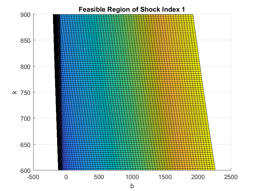
As shown in the figure, the level of bond that gives a same lower bound of consumption (here \(\tilde{c}\) equal to 100) is declining in capital, suggesting that a higher capital allows the current debt to be higher. However, determining this lower bound of bond level is difficult; but determining the boundary condition for consumption is much easier (\(\tilde{c}=0\)).
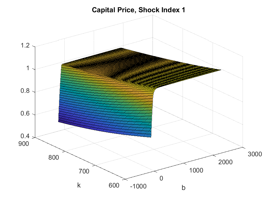
We can inspect the policy functions by projecting them to the natural state space as well. For example, the capital price:
>> figure;
[cTilde_mesh,k_mesh] = ndgrid(IterRslt.var_state.cTilde,IterRslt.var_state.k);
surf(squeeze(IterRslt.var_aux.b(1,:,:)),k_mesh,squeeze(IterRslt.var_aux.q(1,:,:)));
xlabel('b');
ylabel('k');
title('Capital Price, Shock Index 1');
And the multiplier (normalized by marginal utility) for collateral constraint:
>> figure;
[cTilde_mesh,k_mesh] = ndgrid(IterRslt.var_state.cTilde,IterRslt.var_state.k);
surf(squeeze(IterRslt.var_aux.b(1,:,:)),k_mesh,squeeze(IterRslt.var_policy.mu(1,:,:)));
xlabel('b');
ylabel('k');
title('Multiplier for the Collateral Constraint, Shock Index 1');
view(-16,26);
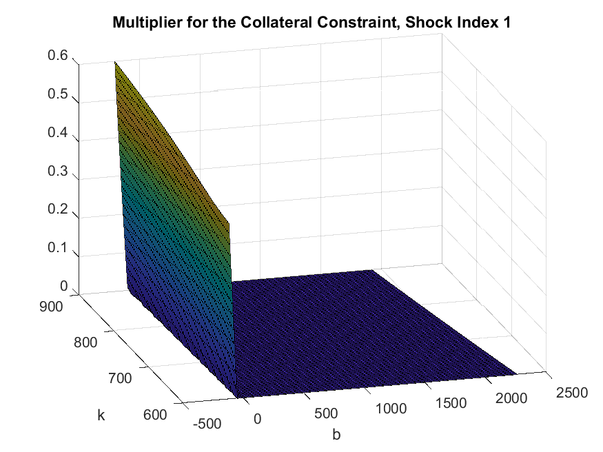
These two policy functions show that the collateral constraint tends to bind when bond is low (borrowing is high). And capital price falls rapidly in borrowing when the collateral constraint binds.
With the converged policy and state transition functions, we can simulate the economy’s ergodic set. To remind readers, here we directly interpolate the state transition and policy functions to simulate, which is faster than resolving the system (the simulation with 24 paths of 50,000 periods completes in less than half a minute on a regular laptop). This is done by specifying in the gmod file
22SIMU_RESOLVE=0; SIMU_INTERP=1; % Use interp for fast simulation
In this case, the variables to be recorded in the simulation need to be explicitly specified in var_output
107var_output c Y cTildeNext q mu inv kNext bNext b v nx gdp b_gdp nx_gdp lev wkcptl;
and can then be included in var_simu
167 var_simu c Y q inv b mu bNext v nx gdp b_gdp nx_gdp lev wkcptl;
With implicit state transition functions for \(\tilde{c}\) solved as part of the policy functions, the transitions need to be specified in the simulate block
168 cTilde' = cTildeNext';
which means that the next period cTilde should pick policy cTildeNext at a sampled exogenous shock index.
Calling simulate_mnendoza2010 produces the following
>> SimuRslt = simulate_mendoza2010(IterRslt);

Periods: 1000
shock  cTilde       k       c       Y       q     inv       b   bNext       v      nx     gdp   b_gdp  nx_gdp     lev  wkcptl
    1   166.9   747.1   282.5     429   1.048   78.98   109.7   86.46   43.32  -23.58   385.9  0.2843 -0.06110.0002417   76.13

...

Periods: 50000
shock  cTilde       k       c       Y       q     inv       b   bNext       v      nx     gdp   b_gdp  nx_gdp     lev  wkcptl
    5   149.8   741.1   262.8   423.8  0.9844   61.04  -33.48  -31.26   42.34   13.19   381.7-0.08769 0.03455 -0.1525    74.4
We can inspect the histogram of the natural state variables \((k,b)\) by calling in MATLAB:
>> figure;
hist3([SimuRslt.b(:),reshape(SimuRslt.k(:,1:end-1),[],1)],[50,50],'CDataMode','auto','FaceColor','interp');
view([15,30]);
xlabel('Bond');
ylabel('Capital');
title('Histogram of Capital and Bond');
print('figures/histogram_b_k.png');
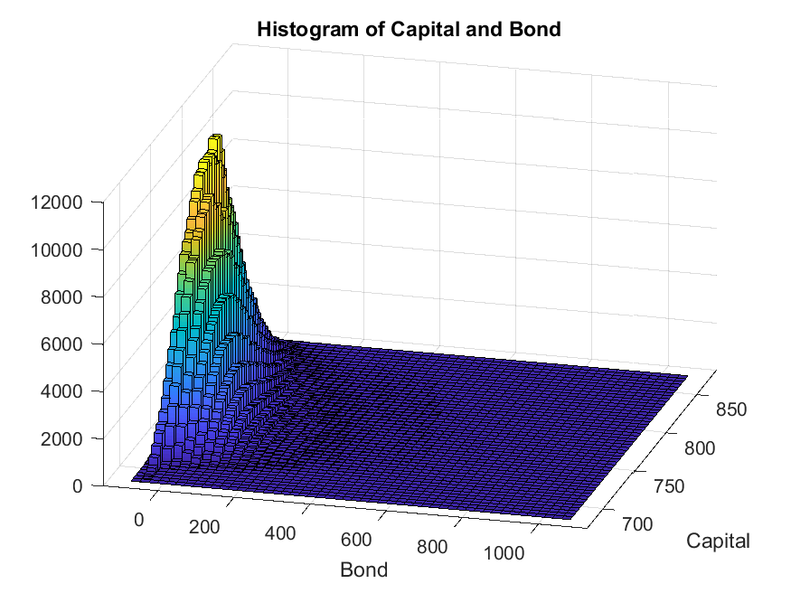
We are interested in the fraction of time that the economy spends in a crisis, i.e., states with binding collateral constraint:
>> muGreaterThanZero = SimuRslt.mu > 1e-7;
fractionCrisis = sum(muGreaterThanZero(:)) / numel(muGreaterThanZero(:));
fprintf('The fraction in crisis: %g\n',fractionCrisis);
The fraction in crisis: 0.131997
We can calculate the unconditional moments:
>> statsList = {'mean','std'};
varList = {'gdp','c','inv','nx_gdp','k','b_gdp','q','lev','v','wkcptl'};
ratioList = {'nx_gdp','b_gdp','lev'};
meanStats = struct;
stdStats = struct;
corrStats = struct;
autoCorrStats = struct;
startPeriod = 1001;
endPeriod = 50000;
for i_var = 1:length(varList)
    varName = varList{i_var};
    meanStats.(varName) = mean(reshape(SimuRslt.(varName)(:,startPeriod:endPeriod),[],1));
    if max(strcmp(varName,ratioList))==1
        stdStats.(varName) = std(reshape(SimuRslt.(varName)(:,startPeriod:endPeriod),[],1));
    else
        stdStats.(varName) = std(reshape(SimuRslt.(varName)(:,startPeriod:endPeriod),[],1)) ...
            / meanStats.(varName);
    end
    corrStats.(varName) = corr(reshape(SimuRslt.(varName)(:,startPeriod:endPeriod),[],1), ...
        reshape(SimuRslt.gdp(:,startPeriod:endPeriod),[],1));
    autoCorrStats.(varName) = corr(reshape(SimuRslt.(varName)(1,startPeriod+1:endPeriod),[],1), ...
        reshape(SimuRslt.(varName)(1,startPeriod:endPeriod-1),[],1));
end
GDSGE |
Mendoza (2010), Table 3, Panel C |
|
Mean |
||
gdp |
400.646 |
388.339 |
c |
277.349 |
267.857 |
inv |
68.838 |
65.802 |
nx/gdp |
0.018 |
0.024 |
k |
780.598 |
747.709 |
b/gdp |
-0.031 |
-0.104 |
q |
1.000 |
1.000 |
leverage |
-0.124 |
-0.159 |
v |
43.268 |
41.949 |
wkcptl |
78.555 |
75.455 |
Std in percent |
||
gdp |
3.88% |
3.85 |
c |
3.68% |
3.69 |
inv |
13.30% |
13.45 |
nx/gdp |
2.67% |
2.58 |
k |
4.32% |
4.31 |
b/gdp |
13.97% |
8.9 |
q |
3.19% |
3.23 |
leverage |
6.53% |
4.07 |
v |
5.85% |
5.84 |
wkcptl |
4.30% |
4.26 |
Corr w/ gdp |
||
gdp |
1.000 |
1.000 |
c |
0.898 |
0.931 |
inv |
0.649 |
0.641 |
nx/gdp |
-0.131 |
-0.184 |
k |
0.753 |
0.744 |
b/gdp |
-0.187 |
-0.298 |
q |
0.408 |
0.406 |
leverage |
-0.174 |
-0.258 |
v |
0.830 |
0.823 |
wkcptl |
0.995 |
0.987 |
Auto corr |
||
gdp |
0.820 |
0.815 |
c |
0.796 |
0.766 |
inv |
0.506 |
0.483 |
nx/gdp |
0.514 |
0.447 |
k |
0.963 |
0.963 |
b/gdp |
0.985 |
0.087 |
q |
0.452 |
0.428 |
leverage |
0.990 |
0.040 |
v |
0.773 |
0.764 |
wkcptl |
0.798 |
0.777 |
Most statistics are similar to Mendoza (2010) except that Mendoza (2010) uses a Stationary Cardinal Utility (SCU) utility function and solves the model by solving a quasi social planner’s problem which produces (1) less persistent leverage and bond, and (2) higher leverage and more negative bond/gdp ratio. These differences are also noted in Mendoza and Villalvazo (2020).
What’s Next?
This example illustrates how to solve a model with two endogenous state variables of which the feasible region may be non-rectangle and hard to determine ex-ante. The crucial step is to transform the boundary condition to that of an endogenous state variable which makes the feasible region a simple rectangle. In the current example, the feasible debt level is high so the model can be solved directly over the natural state space—bond and capital. Such transformation becomes essential for more complex problems, and sometimes the boundary condition needs to be solved using a different equilibrium system. The toolbox accommodates this by allowing a different system of equations for problems at the boundary. See Cao and Nie (2017) for such an example, in which consumption is zero and the Inada condition is violated at the boundary.
The policy functions in the current example are highly nonlinear. We learned how to start with a crude grid and refine the solution with finer grids. A more effective approach is to let the toolbox automatically adapt the grids to increase points in regions that are nonlinear. The example in Bianchi (2011) shows how to use adaptive grids for a model with a single-dimension endogenous state. The current model can also be solved with adaptive grids by simply specifying one option in the gmod file, which we leave as an exercise.
Or you can directly proceed to Toolbox API.