Huggett (1997): Steady States and Transition Paths in Heterogeneous Agent Models

The Model

We use the seminal work Huggett (1997) to illustrate how the toolbox can be used to solve steady states and transition paths of a heterogeneous-agent model. The example also demonstrates how to conduct non-stochastic simulations using the toolbox, by keeping track of the distribution function over a refined grid of individual state variables.

Though the toolbox is not designed for solving the equilibrium of this type of model directly, since the decision problem is characterized by an equation system (the Euler equation

\[u'(c_t) = \beta \mathbb{E}_t[(1+r_{t+1})u'(c_{t+1})] + \lambda_t,\]

where \(\lambda_t\) is the Lagrange multiplier on the borrowing constraint, and the complementary-slackness condition, \(\lambda_t k_{t+1}=0\)) with state transition functions, it readily fits in the toolbox’s general framework. One just needs an extra fixed-point loop to update the aggregate equilibrium object, which can be coded in MATLAB. For the one-sector model studied by Huggett (1997), the steady state aggregate equilibrium object is the aggregate capital stock; the transition path aggregate equilibrium object is the time sequence of the aggregate capital stock.

We directly define the equilibrium, which covers all the ingredients we need for computing the model. For the full description of the model, see Huggett (1997) .

A sequential equilibrium is a time sequence of (1) policy functions \(c_{t}(k,e)\), \(\lambda_t(k,e)\), \(k'_t(k,e)\); (2) measures over individual states \(\phi_t\); (3) aggregate prices and quantities \(w_t, r_t, K_t\), s.t.

1. \(c_t(k,e), \lambda_t(k,e), k_t'(k,e)\) satisfy individuals’ optimality conditions. That is, they solve

\[\begin{split}c_t(k,e)^{-\sigma}=\beta(1+r_{t+1})E[c_{t+1}(k_t'(k,e),e')^{-\sigma} | e] + \lambda_t(k,e), \\ k_t'(k,e)\lambda_t(k,e)=0, \quad \lambda_t(k,e)\geq0, \quad k_t'(k,e)\geq0, \\ c_t(k,e)+k_t'(k,e)=k(1+r_t)+w_te.\end{split}\]

2. Prices are competitively determined and markets clearing:

\[\begin{split}r_t = \alpha K_t^{\alpha-1}-\delta \\ w_t = (1-\alpha) K_t^{\alpha} \\ K_t = \int k \ \phi_t(dk,de)\end{split}\]

3. \(\phi_t\) are consistent with the transitions implied by policy functions and exogenous shocks.

A steady-state equilibrium is a sequential equilibrium with time-invariant equilibrium objects.

Notice we have transformed the individual’s optimization problem into first order conditions and complementarity slackness conditions, which enable us to solve the decision problem with the toolbox.

The gmod File and MATLAB File

huggett1997.gmod

% Toolbox options
INTERP_ORDER = 4; ExtrapOrder = 4;
SIMU_RESOLVE = 0; SIMU_INTERP = 1;
SaveFreq = inf; PrintFreq = 100;
TolEq = 1e-6;
% Parameters
parameters beta sigma kMin r w;
beta = 0.96;    % discount factor
sigma = 1.5;    % CRRA coefficient
alpha = 0.36;   % capital share in production
delta = 0.1;    % depreciation rate

% States
var_state k;
kPts = 100;
kMin = 0;
kMax = 20;
kShift = 1e-3;
k = exp(linspace(log(kMin+1e-3),log(kMax+1e-3),kPts)) - 1e-3;

% Shock process in Huggett (1997)
var_shock e;
e = [0.8, 1.2];
shock_num = 2;
shock_trans = [0.5,0.5;0.5,0.5];

% Representative-agent steady state
kSs = ( (1/beta+delta-1) / alpha )^(1/(alpha-1));
% Initial prices
r = alpha*kSs^(alpha-1) - delta;
w = (1-alpha)*kSs^alpha;

% State transition functions
var_interp Evp_interp;
initial Evp_interp (k.*(1+r)+e.*w).^(-sigma);
% Update
Evp_interp = shock_trans*vp;

% Endogenous variables
var_policy k_next lambda;
inbound k_next kMin k.*(1+r)+e.*w;
inbound lambda 0 1.0;

% Other variables
var_aux c vp;
% Used in simulation
var_output c k_next;
var_others kSs alpha delta output_interp_t;

TASK = 'ss';    % Default task, need overwritten
output_interp_t = {};      % Default transition path;
pre_iter;
  % The pre_iter block will be called at the beginning of every policy iteration
  switch TASK
    case 'ss'
    case 'transition'
      t = T - GDSGE_Iter + 1;  % Convert forward to backward
      r = r_t(t);
      w = w_t(t);
  end
end;

model;
  budget = k*(1+r) + e*w;
  c = budget - k_next;
  up = c^(-sigma);
  [Evp_future] = GDSGE_INTERP_VEC(shock,k_next);
  euler_residual = -1 + beta*Evp_future/up + lambda;
  vp = up*(1+r);    % Envelope theorem
  
  equations;
    euler_residual;
    lambda*(k_next-kMin);
  end;
end;

post_iter;
  % The post_iter block will be called at the end of every policy iteration
  switch TASK
    case 'transition'
      % The following code constructs function approximation for  var_output
      % and stores in IterRslt.output_interp
      OUTPUT_CONSTRUCT_CODE;
      % Store the period-t equilbrium object
      output_interp_t{t} = IterRslt.output_interp;
  end
end;

simulate;
  num_periods = 1;
  num_samples = 10000;
  initial k kSs;    % A place holder
  initial shock 1;  % A place holder
  var_simu c;
  k' = k_next;
end;

The MATLAB file that calls the toolbox codes and manually update equilibrium objects main.m

%% Solve a WarmUp problem
IterRslt = iter_huggett1997;

%% A fixed-point loop to solve the initial steady state
tolEq = 1e-5; metric = inf; iter = 0;
UPDATE_SPEED = 0.01;
K = IterRslt.var_others.kSs;
alpha = IterRslt.var_others.alpha; delta = IterRslt.var_others.delta;
% Non-stochastic simulation, prepare distribution grid
kFinePts = 1000; shockPts = IterRslt.shock_num;
kFine = linspace(min(IterRslt.var_state.k),max(IterRslt.var_state.k),kFinePts)';
kFineRight = [kFine(2:end);inf];
[kFineGrid,shockGrid] = ndgrid(kFine,1:shockPts);
% Parameters to simulate only one step
simuOptions.num_periods = 1;
simuOptions.num_samples = numel(kFineGrid);
simuOptions.init.k = kFineGrid(:);
simuOptions.init.shock = shockGrid(:);
while metric > tolEq
    % Solve at prices implied by current K
    options = struct;
    options.TASK = 'ss';
    options.r = alpha*K^(alpha-1) - delta;
    options.w = (1-alpha)*K^alpha;
    options.WarmUp = IterRslt;
    IterRslt = iter_huggett1997(options);
 
    % Non-stochastic simulation. Simulate one-step to get the state transition
    % functions over kFine
    SimuRslt = simulate_huggett1997(IterRslt,simuOptions);
    % Construct the Markov transition implied by policy functions
    kp = SimuRslt.k(:,2);
    [~,kpCell] = histc(kp, [kFine;inf]);
    leftWeights = (kFineRight(kpCell)-kp) ./ (kFineRight(kpCell)-kFine(kpCell));
    leftWeights(kpCell>=kFinePts) = 1;
    rowVec = [1:shockPts*kFinePts]';
    transToKp = sparse(rowVec,kpCell,leftWeights,shockPts*kFinePts,kFinePts) ...
        + sparse(rowVec(kpCell<kFinePts),kpCell(kpCell<kFinePts)+1,1-leftWeights(kpCell<kFinePts),...
        shockPts*kFinePts,kFinePts);
    % Accomodate the exogenous transition
    transFull = repmat(transToKp,[1,2]) * 0.5;
    % Simulate
    [stationaryDist,~] = eigs(transFull',1,1);
    stationaryDist = reshape(stationaryDist / sum(stationaryDist(:)),[kFinePts,shockPts]);
    % Statistics
    K_new = sum(reshape(stationaryDist.*reshape(kFine,[kFinePts,1]), [], 1));

    % Update
    metric = abs(log(K) - log(K_new));
    iter = iter + 1;
    fprintf('Steady-state iterations: %d, %g\n',iter, metric);
    fprintf('===============================\n');
    K = K_new*UPDATE_SPEED + K*(1-UPDATE_SPEED);
end

%% Solve the transition path
T = 1000;
K_t = K*ones(1,T);
K_t_new = K*ones(1,T);
tolEq = 1e-3; metric = inf; iter = 0;
UPDATE_SPEED = 0.01;
% Initial distribution in Huggett (1997)
dist0 = stationaryDist;
dist0(1,:) = 0.2/2;
kBar = K/0.8*2;
kBarIndex = find(kFine>kBar,1);
dist0(2:kBarIndex,:) = 0.8 / numel(dist0(2:kBarIndex,:));
dist0(kBarIndex+1:end,:) = 0;
while metric > tolEq
    % Backward loop
    options = struct;
    options.TASK = 'transition';
    options.PrintFreq = inf;
    options.MaxIter = T;
    options.T = T;
    options.TolEq = 0;  % Do not check TolEq
    options.r_t = alpha*K_t.^(alpha-1) - delta;
    options.w_t = (1-alpha)*K_t.^alpha;
    options.WarmUp = IterRslt;  % Start from steady state
    options.WarmUp.Iter = 0;    % Start with iter 0;
    IterRslt_t = iter_huggett1997(options);

    % Forward simulation
    dist = dist0;
    for t=1:1:T
        K_t_new(t) = sum(reshape(dist.*reshape(kFine,[kFinePts,1]), [], 1));
        % Simulate using period-t policies
        IterRslt.output_interp = IterRslt_t.var_others.output_interp_t{t};
        SimuRslt_t = simulate_huggett1997(IterRslt,simuOptions);
        % Construct the Markov transition implied by policy functions
        kp = SimuRslt_t.k(:,2);
        [~,kpCell] = histc(kp, [kFine;inf]);
        leftWeights = (kFineRight(kpCell)-kp) ./ (kFineRight(kpCell)-kFine(kpCell));
        leftWeights(kpCell>=kFinePts) = 1;
        rowVec = [1:shockPts*kFinePts]';
        transToKp = sparse(rowVec,kpCell,leftWeights,shockPts*kFinePts,kFinePts) ...
            + sparse(rowVec(kpCell<kFinePts),kpCell(kpCell<kFinePts)+1,1-leftWeights(kpCell<kFinePts),...
            shockPts*kFinePts,kFinePts);
        % Accomodate the exogenous transition
        transFull = [transToKp,transToKp] * 0.5;
        dist = reshape(dist(:)'*transFull,[kFinePts,shockPts]);
    end
    
    % Update K_t
    metric = max(abs(log(K_t) - log(K_t_new)));
    iter = iter + 1;
    fprintf('Transition path iterations: %d, %g\n',iter, metric);
    fprintf('==================================\n');
    if metric<2e-2
        UPDATE_SPEED = 0.03;
    end
    K_t = K_t_new*UPDATE_SPEED + K_t*(1-UPDATE_SPEED);
end

%% Plot
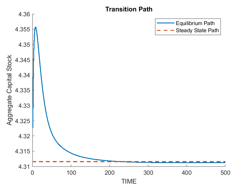
figure; hold on;
plot(K_t(1:500),'LineWidth',1.5);
plot([0,500],[K,K],'--','LineWidth',1.5);
title('Transition Path');
xlabel('TIME');
legend({'Equilibrium Path','Steady State Path'});
ylabel('Aggregate Capital Stock');
print('transition_path.png','-dpng');

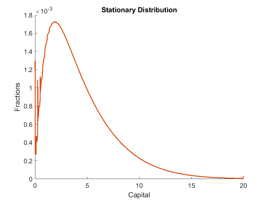
figure; hold on;
plot(kFine,stationaryDist,'LineWidth',1.5);
title('Stationary Distribution');
xlim([0,20]);
xlabel('Capital');
ylabel('Fractions');
print('stationary_dist.png','-dpng');

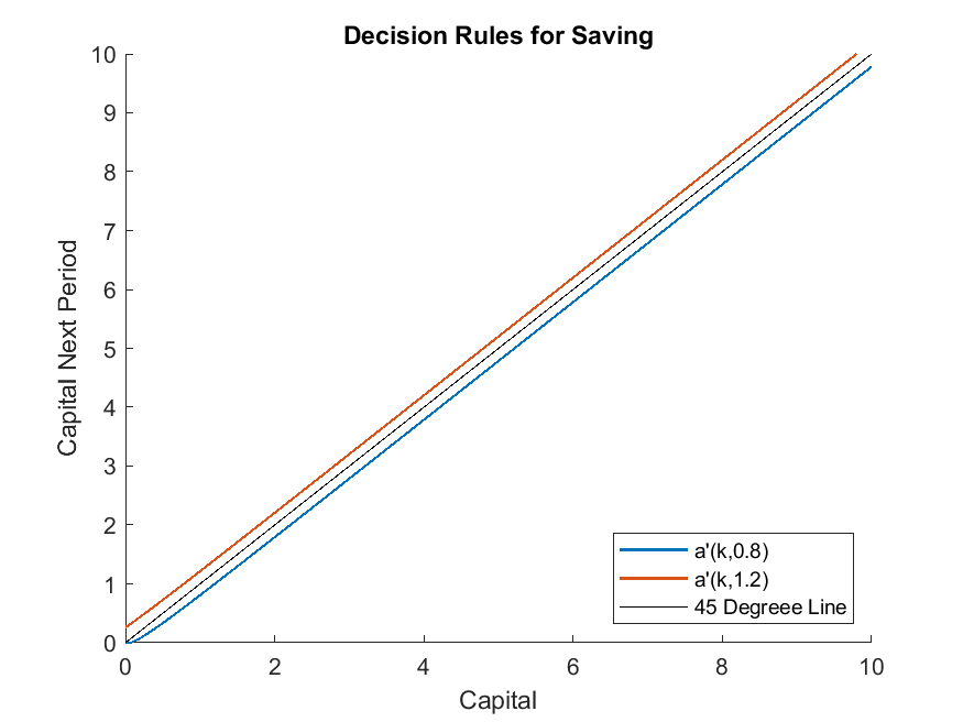
figure; hold on;
plot(IterRslt.var_state.k,IterRslt.var_policy.k_next,'LineWidth',1.0);
plot(IterRslt.var_state.k,IterRslt.var_state.k,'k-');
xlim([0,10]);
ylim([0,10]);
legend('a''(k,0.8)','a''(k,1.2)','45 Degreee Line','Location','SouthEast');
xlabel('Capital');
ylabel('Capital Next Period');
title('Decision Rules for Saving');
print('policy_function_kp.png','-dpng');

Output

The code produces the stationary distribution

the transition path starting from an equal wealth distribution (see the MATLAB file for how the initial distribution is constructed)

and the policy functions at the steady state.