Brumm et al (2015): A GDSGE model with asset price bubble

Brumm, Grill, Kubler, and Schmedders (2015) study a GDSGE model with multiple assets with different degrees of collaterability. They find that a long-lived asset that never pays dividend but can be used as collateral to borrow can have strictly positive price in equilibrium. From the traditional asset-pricing point of view, this positive price is a bubble because the present discounted value of dividend from the asset is exactly zero.

The model is similar to the ones in Heaton and Lucas (1996) and Cao (2018). It features two representative agents \(h\in\{1,2\}\) who have Epstein-Zin utility with the same intertemporal elasticity of substitution and different coefficients of risk-aversion:

\[U_{h,t}=\left\{\left[c_{h,t}\right]^{\rho^h}+\beta\left[\mathbb{E}_{t}\left(U_{h,t+1}^{\alpha^h}\right)\right]^{\frac{\rho^h}{\alpha^h}}\right\}^{\frac{1}{\rho^h}}.\]

The agents can trade in shares of two long-lived assets (Lucas’ trees), \(i\in\{1,2\}\) and a risk-free bond.

In period \(t\) (we suppress the explicit dependence on shock history \(z^t\) to simplify the notation), asset \(i\) pays dividend \(d_{i,t}\) worth a fraction \(\sigma_i\) of aggregate output and traded at price \(q_{i,t}\). The agents cannot short sell the long-lived asset but they can short sell the risk-free bond, i.e., borrow. In order to borrow in the risk-free bond, the agents must use the assets as collateral. The agents can pledge a fraction \(\delta_i\) of the value of their asset \(i\) holding as collateral. In particular, the collateral constraint takes the form:

\[\phi^h_{t+1}+\sum_{i\in\{1,2\}}\theta^h_{i,t+1}\delta_i\min_{z^{t+1}|z^t}(q_{i,t+1}+d_{i,t+1})\geq0,\]

where \(\phi^h,\theta^h_1,\theta^h_2\) denote the bond holding, and asset \(1\) and asset \(2\) holdings of agents \(h\).

This model can be written and solved using our toolbox. This is done by Hewei Shen from the University of Oklahoma, who generously contributed the GDSGE code below. Hewei’s own research demonstrates the importance of GDSGE models in studying macro-prudential and fiscal policies in emerging market economies, such as his recent publication and his ongoing work with Siming Liu from Shanghai University of Finance and Economics.

Notice that in the GDSGE code, asset \(1\) never pays dividend, i.e., \(\sigma_1 = 0\). Therefore, in finite-horizon economies, by backward induction, its price is always equal to \(0\). In order for the sequence of finite-horizon equilibria to converge to an infinite-horizon equilibrium in which asset \(1\) has positive price, we need to assume that agents derive utility from holding the asset in the very last period in each T-period economy:

\[U_{h,T} = \left[c_{h,T}\right]^{\rho^h}+\zeta \left[\theta^h_{1,T}\right]^{\rho^h}.\]

This assumption is a purely numerical device and becomes immaterial when \(T\rightarrow\infty\). To solve the last period problem, we use a model_init block that has a different system of equations than that of the main model block (see Cao and Nie (2017) for another example using a different model_init).

The gmod File

BGKS2015.gmod

%Options
SolMaxIter=20000;
PrintFreq=200;
SaveFreq =200;
USE_SPLINE=1;
INTERP_ORDER=2;


% Parameters
parameters beta alpha1 alpha2 rho1 rho2 e1 e2 sigma1 sigma2 d1 d2 delta1 delta2 zeta
zeta = 10; %utility from holding asset 1
% which only applies in the very last period of finite horizon economies
beta=0.977; %subjective discount factors
alpha1=0.5; % RA of agent 1 = 0.5
alpha2=-6; % RA of agent 2 = 7
rho1=0.5; % IES=2
rho2=0.5; % IES=2
e1=0.085; % agent 1 income share
e2=0.765; % agent 2 income share
sigma1=0.0; % Tree 1 dividend share, here =0. Tree 1 has no intrinsic value
sigma2=0.15; % Tree 2 dividend share
d1=sigma1; % Tree 1 dividend
d2=sigma2; % Tree 2 dividend
delta1=1; % Tree 1 collateralizability
delta2=0; % Tree 2 collateralizability


% Shock variables
var_shock g; %aggregate endowment growth rate

% Shocks and transition matrix
shock_num = 4;
g = [0.72, 0.967, 1.027, 1.087 ]; 
shock_trans = [
  0.022, 0.054, 0.870, 0.054
  0.022, 0.054, 0.870, 0.054
  0.022, 0.054, 0.870, 0.054
  0.022, 0.054, 0.870, 0.054
  ];


% State variables
var_state w1;  % wealth share
w1 = linspace(0,1,240);

% Variable for the last period
var_policy_init c1 c2 q1 theta11;

inbound_init theta11 0 1; %agent 1: tree 1 holding, constrained by no-short selling condition
inbound_init q1 0 100;
inbound_init c1 1e-10 1;
inbound_init c2 1e-10 1;

var_aux_init v1 v2;

model_init;
  budget_1 = c1 + theta11*q1 - e1 - w1*(q1+ d1 +d2);
  FOC1 = c1^(rho1-1)-q1*zeta*theta11^(rho1-1);
  FOC2 = c2^(rho2-1)-q1*zeta*(1-theta11)^(rho2-1);  
  v1 =(c1^(rho1)+ zeta*theta11^(rho1))^(1/(rho1));
  v2 =(c2^(rho2)+ zeta*(1-theta11)^(rho2))^(1/(rho2));
  equations;
    budget_1;
    c1+c2-1;
    FOC1;
    FOC2;
  end;
end;

% Endogenous variables and bounds
var_policy c1 c2 theta11 theta21 nphi1 nphi2 mu_theta11 mu_theta21 mu_theta12 mu_theta22 muphi1 muphi2 q1 q2 p w1n[4];
inbound c1 1e-10 1;
inbound c2 1e-10 1;
inbound theta11 0 1; %agent 1: tree 1 holding, constrained by no-short selling condition
inbound theta21 0 1; %agent 1: tree 2 holding, constrained by no-short selling condition
inbound nphi1 0 100;
inbound nphi2 0 100;
inbound mu_theta11 0 100; %multipliers on no-short selling constraint on trees
inbound mu_theta21 0 100;
inbound mu_theta12 0 100;
inbound mu_theta22 0 100;
inbound muphi1 0 100; %multipliers on the bond position
inbound muphi2 0 100; 
inbound q1 0 100;
inbound q2 0 100;
inbound p 0 100;
inbound w1n -0.05 1.05 adaptive(2);

% Extra output variables
var_aux phi1 phi2 theta12 theta22 v1 v2 collat_premium;

% Interpolation objects
var_interp c1p c2p v1p v2p q1p q2p pp;

% Initialize using model_init
initial c1p c1;
initial c2p c2;
initial v1p v1;
initial v2p v2;
initial q1p q1;
initial q2p 0;
initial pp 0.0;

% Time iterations update
c1p = c1;
c2p = c2;
v1p = v1;
v2p = v2;
q1p = q1;
q2p = q2;
pp = p;

% Variables to be used in simulation if SIMU_RESOLVE=1
var_output c1 c2 v1 v2 theta11 theta21 theta12 theta22 phi1 phi2 q1 q2 p collat_premium w1n;

model;
  % Interpolation
  [c1p',c2p', v1p', v2p', q1p', q2p', pp'] = GDSGE_INTERP_VEC'(w1n');

  % Expectations
  ev1 = GDSGE_EXPECT{ (g'*v1p')^(alpha1)};
  ev2 = GDSGE_EXPECT{ (g'*v2p')^(alpha2)};
  expuc1 = GDSGE_EXPECT{ (g'^alpha1)*(v1p'^(alpha1-rho1))*((c1p'/c1)^(rho1-1))/g'};
  expuc2 = GDSGE_EXPECT{ (g'^alpha2)*(v2p'^(alpha2-rho2))*((c2p'/c2)^(rho2-1))/g'};
  expucq1h= GDSGE_EXPECT{ (g'^alpha1)*(v1p'^(alpha1-rho1))*((c1p'/c1)^(rho1-1))*(q1p' + d1)};
  expucq1f= GDSGE_EXPECT{ (g'^alpha2)*(v2p'^(alpha2-rho2))*((c2p'/c2)^(rho2-1))*(q1p' + d1)};
  expucq2h= GDSGE_EXPECT{ (g'^alpha1)*(v1p'^(alpha1-rho1))*((c1p'/c1)^(rho1-1))*(q2p' + d2)};
  expucq2f= GDSGE_EXPECT{ (g'^alpha2)*(v2p'^(alpha2-rho2))*((c2p'/c2)^(rho2-1))*(q2p' + d2)};
  q1p_min = GDSGE_MIN{q1p'};
  q2p_min = GDSGE_MIN{q2p'};
  g_min = GDSGE_MIN{g'};

  % bond transformation
  theta12=1-theta11; %calculate the tree holding for agent 2
  theta22=1-theta21;
  collat1= delta1*theta11*(q1p_min+d1) + delta2*theta21*(q2p_min+d2); %collateral values
  collat2= delta1*theta12*(q1p_min+d1) + delta2*theta22*(q2p_min+d2);
  phi1 = (nphi1 - collat1)*g_min; %back out the bond holdings
  phi2 = (nphi2 - collat2)*g_min;

  %Euler Equations
  EE1_q1= beta*(ev1^((rho1-alpha1)/(alpha1)))*expucq1h + muphi1*delta1*g_min*(q1p_min + d1)+ mu_theta11-q1;
  EE1_q2= beta*(ev1^((rho1-alpha1)/(alpha1)))*expucq2h + muphi1*delta2*g_min*(q2p_min + d2)+ mu_theta21 - q2;
  EE1_p= beta*(ev1^((rho1-alpha1)/(alpha1)))*expuc1 + muphi1 -p ;
  EE2_q1= beta*(ev2^((rho2-alpha2)/(alpha2)))*expucq1f + muphi2*delta1*g_min*(q1p_min + d1)+ mu_theta12-q1;
  EE2_q2= beta*(ev2^((rho2-alpha2)/(alpha2)))*expucq2f + muphi2*delta2*g_min*(q2p_min + d2)+ mu_theta22- q2;
  EE2_p= beta*(ev2^((rho2-alpha2)/(alpha2)))*expuc2 + muphi2-p;

  % Budget constraint agent 1
  budget_1 = c1 + p*phi1 + theta11*q1 + theta21*q2 - e1 - w1*( q1+ q2 +d1 +d2);

  % Consistency
  w1_consis' = ( theta11*(q1p' + d1) + theta21*(q2p' + d2) + phi1/g' )/(q1p' + q2p' + d1 +d2) - w1n';

  % Aux variables
  v1 =( c1^(rho1)+ beta* (ev1^((rho1)/(alpha1))))^(1/(rho1));
  v2 =( c2^(rho2)+ beta* (ev2^((rho2)/(alpha2))))^(1/(rho2));
  collat_premium = (q1 - q2*sigma1/sigma2)/(q1+q2);

  equations;
    EE1_q1;
    EE2_q1;
    EE1_q2;
    EE2_q2;
    EE1_p;
    EE2_p;
    phi1+phi2;
    nphi1*muphi1;
    nphi2*muphi2;   
    mu_theta11*theta11;
    mu_theta21*theta21;
    mu_theta12*theta12;
    mu_theta22*theta22;
    budget_1;
    c1+c2-1;
    w1_consis';
  end;
end;

simulate;
  num_periods = 10000;
  num_samples = 100;
  initial w1 0.5;
  initial shock 1;
  var_simu c1 c2 theta11 theta21 theta12 theta22 phi1 phi2 q1 q2 p collat_premium;
  w1' = w1n';
end;

Results

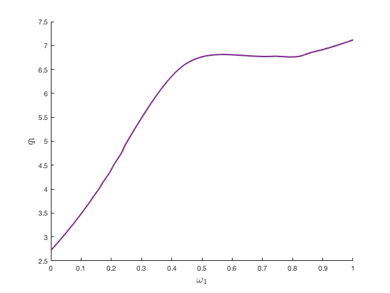
In this example, agents \(1\) (\(\alpha_1 = 0.5\)) are less risk-averse than agents \(2\) (\(\alpha_2 = -6\)) so they tend to borrow to invest in the risky assets \(1\) and \(2\). Asset \(1\) nevers pays dividend (\(\sigma_1=0\)) but can be used as collateral to borrow (\(\delta_1 = 1\)). While asset \(2\) pays dividend (\(\sigma_2>0\)) but cannot be used as collateral (\(\delta_2=0\)). In equilibrium, asset \(1\) still commands a positive price. Therefore, this is an asset price bubble arising from collaterability. The following figure shows the price of asset \(1\) relative to aggregate output as a function of agents \(1\)’s wealth share

\[\omega^1_t = \frac{\theta^1_{1,t}(q_{1,t}+d_{1,t})+\theta^1_{2,t}(q_{2,t}+d_{2,t})+\phi^1_t}{q_{1,t}+d_{1,t}+q_{2,t}+d_{2,t}}.\]

The price of asset \(1\) be as high as several times aggregate output and tends to be higher when agents \(1\) are relatively richer.